Wavelets and adaptive data analysis

21 Oct 2017

For data that have a high signal-to-noise ratio, a nonparametric, adaptive method might be appropriate. In particular, we may want to fit the data to functions that are spatially imhomogenous, i.e., the smoothness of the function \(f(x)\) varies a lot with \(x\).

In this post, we will discuss wavelets, which can be used an adaptive nonparametric estimation method. First, we will introduce some background on function spaces and Fourier transforms, and then we will discuss Haar wavelets, a specific type of wavelet, and how to construct wavelets in general. This presentation follows Wasserman [2], but I’ve included some additional code and images.

Preliminaries

Function spaces

Let \(L_2(a,b)\) denote the set of functions \(f : [a,b] \rightarrow \mathbb{R}\) such that \[ \int_a^b f^2(x) dx < \infty.\] For our purposes, we will assume \(a=0,b=1\). The inner product of \(f,g \in L_2(a,b)\) is defined as \[ \langle f,g \rangle := \int_a^b f(x) g(x) dx, \] and the norm of \(f\) is defined as \[ || f || = \left( \int_a^b f^2(x) dx \right)^{\frac{1}{2}}. \] A sequence of functions \(\phi_1,\phi_2,\ldots\) is orthonormal if \(||\phi_j|| = 1 \) for all \(j\) (i.e., has norm 1), and \( \int_a^b \phi_i(x) \phi_j(x) dx = 0, \,\, i \neq j\) (i.e., orthogonal).

A complete (i.e., the only function orthogonal to each \(\phi_j\) is the 0 function) and orthonormal set of functions form a basis, i.e., if \(f \in L_2(a,b)\), then \(f\) can be expanded in the basis in the following way: \[ f(x) = \sum_{j=1}^\infty \theta_j \phi_j(x), \] where \(\theta_j = \int_a^b f(x) \phi_j(x) dx \).

Sparse functions and Fourier transforms

A function \(f = \sum_j \beta_j \phi_j \) is sparse in a basis \(\phi_1,\phi_2,\ldots\) if most of the \(\beta_j\)’s are 0 or close to 0. Sparseness can be seen as a generalization of smoothness, i.e., a smooth function is sparse, but there are also nonsmooth functions that are sparse.

Let \(f^{*}\) denote the Fourier transform of a function \(f\): \[ f^{*}(t) = \int_{-\infty}^\infty \exp(-ixt) \, f(x) \,dx.\] We can recover \(f\) at almost all \(x\) using the inverse Fourier transform: \[ f(x) = \frac{1}{2\pi} \int_{-\infty}^\infty \exp(ixt) \, f^*(t) \,dt, \] assuming that \(f^{*}\) is absolutely integrable.

Throughout our discussion of wavelets, we will use the following notation: given any function \(f\) and \(j,k \in \mathbb{Z}\), define \[ f_{jk}(x) = 2^{\frac{j}{2}} \, f(2^j x - k). \]

Wavelets

We now turn our attention to wavelets, beginning with the simplest type of wavelet, the Haar wavelet.

Haar wavelet

Haar wavelets are a simple type of wavelet given in terms of step-functions. Specifically, these wavelets are expressed in terms of the the Father and Mother Haar wavelets. Our goal is to define an orthonormal basis for \(L_2([0,1])\)—to do so, we need to introduce the Father and Mother wavelets and their shifted and rescaled sets.

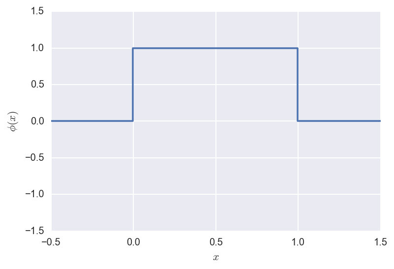
The Father wavelet is defined as:

\[\phi(x) = \begin{cases} 1 &\text{ if } x \in [0,1] \\ 0 &\text{ otherwise } \\ \end{cases}\]

and looks like:

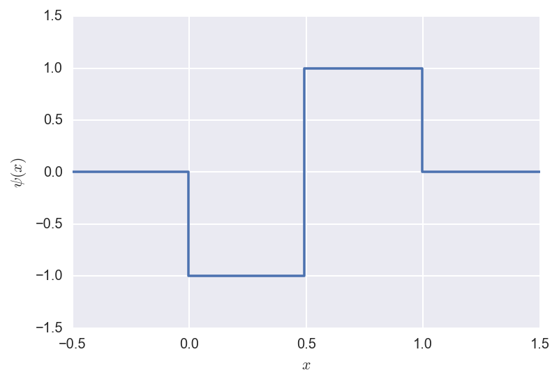
The Mother wavelet is defined as:

\[\psi(x) = \begin{cases} -1 &\mathrm{~if~} x \in [0,1/2] \\ 1 &\mathrm{~if~} x \in (1/2,1] \\ 0 &\mathrm{~otherwise~} \\ \end{cases}\]

and looks like:

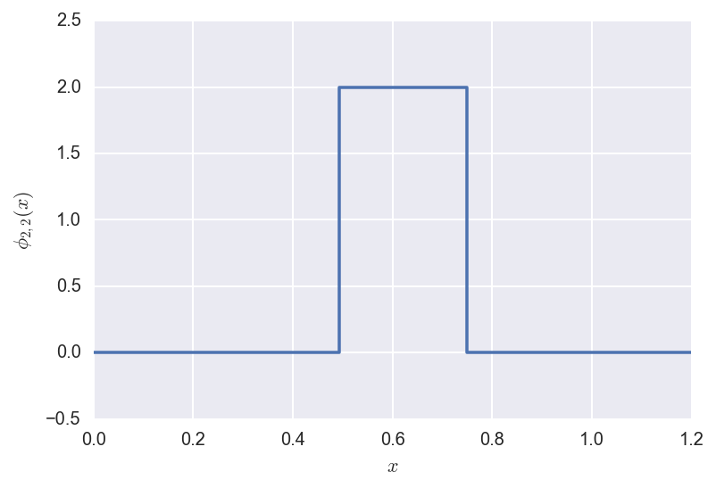
Now we define the wavelets as shifted and rescaled versions of the Father and Mother wavelets, as above:

\[\phi_{jk}(x) = 2^{j/2} \phi(2^j x - k)\]

and

\[\psi_{jk}(x) = 2^{j/2} \psi(2^j x - k).\]

Below we plot some examples.

The shifted/rescaled father wavelet \(\phi_{2,2}\) looks like:

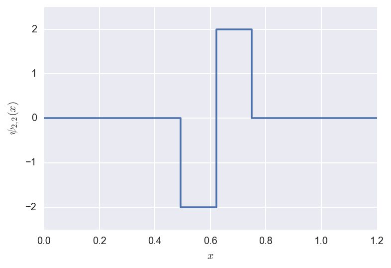
The shifted/rescaled mother wavelet \(\psi_{2,2}\) looks like:

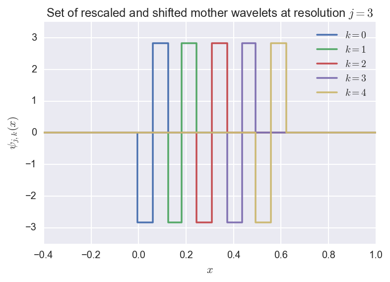
Now we define the set of rescaled and shifted mother wavelets at resolution $j$ is defined as: \(W_j = \{\psi_{jk}, k=0,1,\ldots,2^{j-1}\}.\)

We plot an example where \(j=3\):

The next theorem defines gives an orthonormal basis for \(L_2(0,1)\) in terms of the introduced sets, which allows us to write any function in this space as a linear combination of the basis elements.

Theorem: The set of functions \(\{\phi, W_0, W_2, W_2,\ldots\}\) is an orthonormal basis for \(L_2(0,1)\), i.e., the set of real-valued functions on \([0,1]\) where \(\int_0^1 f^2(x) dx < \infty\).

As a result, we can expand any function \(f \in L_2(0,1)\) in this basis:

\[f(x) = \alpha \phi(x) + \sum_{j=0}^{\infty} \sum_{k=0}^{2^j-1} \beta_{jk} \phi_{jk}(x),\]

where \(\alpha = \int_0^1 \phi(x) dx\) is the scaling coefficient, and \(\beta_{jk} = \int_0^1 f(x) \psi_{jk}(x) dx\) are the detail coefficients.

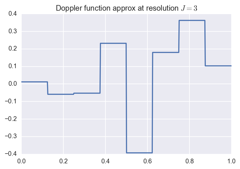
So to approximate a function \(f \in L_2(0,1)\), we can take the finite sum

\[f_J(x) = \alpha \phi(x) + \sum_{j=0}^{J-1} \sum_{k=0}^{2^j-1} \beta_{jk} \phi_{jk}(x).\]

This is called the resolution \(J\) approximation, and has \(2^J\) terms.

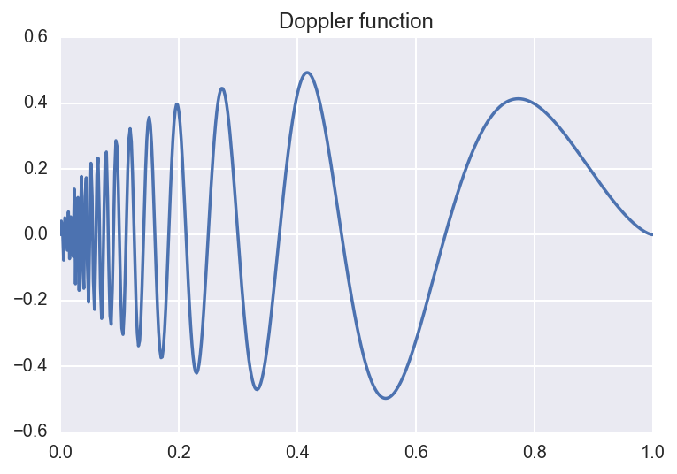
We consider an example below. Suppose we are interested in approximating the Doppler function:

\[f(x) = \sqrt{x (1-x)} \, \sin(\frac{2.1 \pi}{x + 0.05}).\]

We can approximate this function by considering several resolutions (i.e., finite truncations of the wavelet expansion sum). Below, we plot the original function along with the resolution \(J=3,5,8\) approximations:

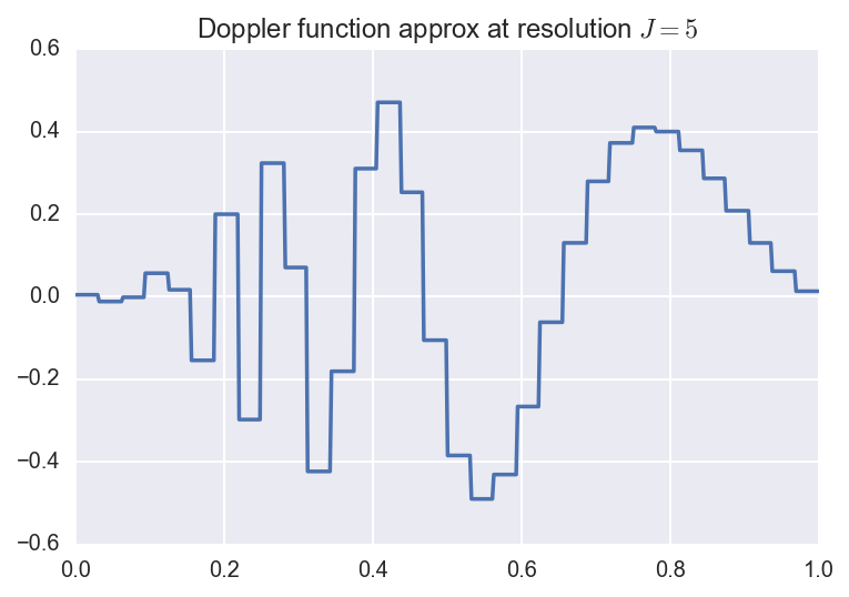
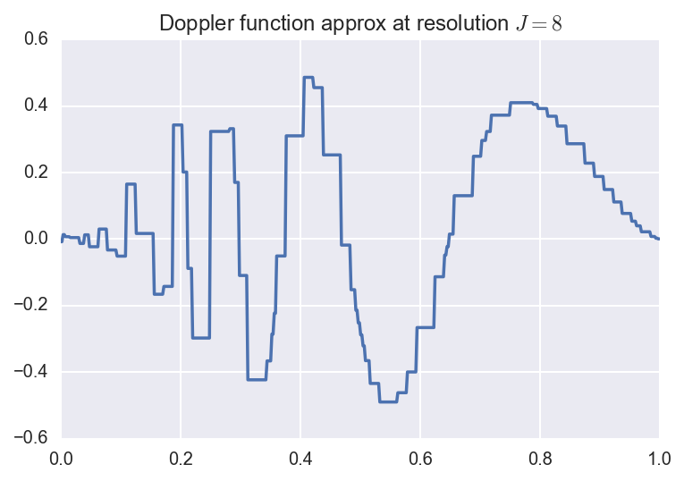
Here, the coefficients were computed using numerical quadrature. Below, we plot the resolution \(J=5\) approximation along with the coefficients. The \(y\)-axis represents which resolution or level the coefficient comes from. The height of the bars are proportional to the size of the coefficients, and the direction of the bar corresponds to the sign of the coefficient.

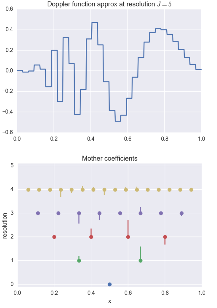
For instance, for certain applications, the \(x\)-axis could be represent time, and the resolutions could then be interpreted as sub-intervals of time.

Constructing smooth wavelets

Haar wavelets are simple to describe and are localized, i.e., the mass is concentrated in one area. We can express these same ideas for more general functions, which can give us approximations that are smooth and localized. Intuitively, it is useful to consider these specific concepts in terms of Haar wavelets, and to know that we can use these ideas for more general functions \(\phi\) in the following way.

Given any function \(\phi\), we can define the subspaces of \(L_2(\mathbb{R})\) as follows:

\[\begin{align} V_0 &= \left\{ \,f \,\,\bigl|\,\, f(x) = \sum_{k \in \mathbb{Z}} c_k \,\phi(x - k), \sum_{k \in \mathbb{Z}} c_k^2 \infty \right\} \\ V_1 &= \left\{ \,f(x) = g(2x) \,\,\bigl|\,\, g \in V_0 \right\} \\ V_2 &= \left\{ \,f(x) = g(2x) \,\,\bigl|\,\, g \in V_1 \right\} \\ \vdots \end{align}\]

Definition: We say that \(\phi\) generates a multiresolution analysis (MRA) of \(\mathbb{R}\) if

\[V_j \subset V_{j+1}, j\geq 0\]

and

\[\bigcup_{j \geq 0} V_j \mathrm{~is~dense~in~} L_2(\mathbb{R}),\]

i.e., for any function \(f \in L_2(\mathbb{R})\), there exists a sequence of functions \(f_1, f_2, \ldots\) such that each \(f_r \in \bigcup_{j \geq 0} V_j\) and \(||f_r - f|| \rightarrow 0\) as \(r \rightarrow \infty\).

In other words, (…)

Lemma: If \(V_0, V_1, V_2, \ldots\) is an MRA generated by \(\phi\), then

\[\{ \phi_{jk}, k \in \mathbb{Z} \}\]

is an orthonormal basis for \(V_j\).

As an example, we consider the father Haar wavelet as the function \(\phi\). The the MRA generated by \(\phi\) is given by \(\{\phi, V_0, V_1,\ldots\}\), where each \(V_j\) is the set of functions \(f \in L_2(\mathbb{R})\) that are piecewise constant on the interval

\[[k2^{-j}, (k+1) 2^{-j}],\]

for \(k \in \mathbb{Z}\).

Code

Code (Jupyter/iPython notebook) for generating these plots is available on Github.

References

1. W. Härdle, G. Kerkyacharian, D. Picard, A. Tsybakov. Wavelets, Approximation, and Statistical Applications.
2. L. Wasserman. All of Nonparametric Statistics. Chapter 9.