Solving large linear systems with conjugate gradient
31 Aug 2018Why use iterative methods?
One of the most fundamental math problems is solving a linear system: \[ Ax = b, \] where \(A \in \mathbb{R}^{n \times m}\) is a matrix, and \(x \in \mathbb{R}^n\) and \(b \in \mathbb{R}^m\) are vectors; we are interested in the solution, \[ \tilde x = A^{-1} b, \] given by the matrix-vector product of the pseudoinverse of the matrix \(A\) and the vector \(b\).
Now, for the rest of this post, we’ll consider the case where the number of rows and columns are equal, i.e., \(n=m\) and further assume that \(A\) is a symmetric, positive definite (s.p.d.) matrix. This guarantees that an inverse exists.
Typically (without making assumptions on the structure or sparsity of the matrix), matrix inversion via Gaussian elimination (a.k.a. LU factorization) requires \(O(n^3)\) computation. There are many other types of matrix factorization algorithms, including the Cholesky decomposition, which applies to s.p.d. matrices that can be used to solve the problem. However, when the dimension of the problem is very large—for instance, on the order of millions or even larger—matrix factorization becomes too computationally expensive. Trefethen and Bau [3, pp. 243] give the following dates and sizes for what was considered “large” in terms of so-called direct, dense matrix inversion methods:
- 1950: \(n = 20\) (Wilkinson)
- 1965: \(n = 200\) (Forsythe and Moler)
- 1980: \(n = 2000\) (LINPACK)
- 1995: \(n = 20000\) (LAPACK) - LAPACK remains a popular for linear algebra computations today.
Some problems where large linear systems that come up in practice include Kalman filters, problems large covariance matrices (e.g., in genetics), large kernel matrices the size of the square of the number of data points, large regression problems, spectral methods for large graphs.
In these cases, iterative methods, such as conjugate gradient, are popular, especially when the matrix \(A\) is sparse. In direct matrix inversion methods, there are typically \(O(n)\) steps, each requiring \(O(n^2)\) computation; iterative methods aim to cut down on the running time of each of these numbers, and the performance typically depends on the spectral properties of the matrix.
In this post, we’ll give an overview of the linear conjugate gradient method, and discuss some scenarios where it does very well, and others where it falls short.
The conjugate gradient algorithm
The basic idea of conjugate gradient is to find a set of \(n\) conjugate direction vectors, i.e., a set of vectors \(p_1,\ldots,p_n\) satisfying
\[ p_i \, A \, p_j = 0, \quad \forall i \neq j. \]
This set of vectors has the property of being linearly independent and spanning \(\mathbb{R}^n\).
Before discussing the conjugate gradient algorithm, we’ll first present the conjugate directions algorithm, which assumes that we are given a set of \(n\) conjugate vectors. Then we’ll see that conjugate gradient is just a special type of conjugate directions algorithm that can generate the next conjugate vector using only the current vector, a property which gives rise to its computational efficiency.
Conjugate directions algorithm
Suppose we are given the set of conjugate vectors \(p_1,\ldots,p_n\). The conjugate directions algorithm constructs iterates stepping in these directions:
\[ x_{k+1} = x_k + \alpha_k p_k,\]
where \(p_k\) is the \(k\)th conjugate direction, and the step size \(\alpha_k\) is obtained as the minimizer of the convex quadratic equation along \(x_k + \alpha p_k\):
\[ \phi(x) = \frac{1}{2} x^\top A x - b x.\]
Note that the gradient of this equation recovers the solution of original equation of interest
\[ \nabla \phi(x) = A x - b =: r(x).\]
The above equation, which we define as \(r(x)\) is called the residual. Furthermore, define the residual at iterate \(x_k\) as \(r_k := r(x_k)\).
The explicit step-size is given by
\[ \alpha_k = -\frac{ r_k^\top \, p_k }{p_k \, A \, p_k}.\]
Properties of the conjugate directions algorithm
Below, we list two properties that hold for any conjugate directions algorithm. The proofs are in Theorem 5.1 and Theorem 5.2 of Nocedal and Wright [2].
Conjugate directions converges in at most \(n\) steps
An important result is the following: any sequence of vectors generated by the conjugate direction algorithm converges to the solution \(\tilde x\) in at most \(n\) steps.
Expanding subspace minimization
Another important property is that the residual at the current iterate, \(r_k\), is orthogonal to all previous conjugate vectors: i.e.,
\[ r_k^\top p_i = 0, \quad \forall i=0,\ldots,k-1.\]
Furthermore, each iterate \(x_k\) is the minimizer of the quadratic function \(\phi\) over the set defined by vectors in the span of the previous search directions plus the initial point:
\[ \{ x : x = x_0 + \mathrm{span}(p_0, \ldots, p_{k-1})\} .\]
Conjugate gradient algorithm
How do generate a set of conjugate directions? Methods such as computing the eigenvectors (which are conjugate) of \(A\) are expensive. The conjugate gradient algorithm generates a new \( p_{k+1}\) using the vector \(p_k\) with the property that it is conjugate to all existing vectors. As a result, little computation or storage is needed for this algorithm.
The initial conjugate vector \(p_0\) is set to the negative residual at the initial point, i.e., \(p_0 = - r_0 \); recall that the residual is defined to be the gradient of the quadratic objective function, and so, this is the direction of steepest descent.
Each subsequent point is a linear combination of the negative residual \(-r_k\) and the previous direction \(p_{k-1}\):
\[ p_k = -r_k + \beta_k \, p_{k-1}, \]
where the scalar
\[ \beta_k = \frac{r_k^\top A p_{k-1}}{p_{k-1}^\top A p_{k-1}} \]
is such that the vector \(p_k\) along with the previous search directions are conjugate. The above expression for \(\beta_k\) is obtained by premultiplying \(p_k\) by \(p_{k-1} A\) and the condition that \( p_{k-1}^\top A p_k = 0 \).
The final algorithm for conjugate gradient involves a few more simplifications. First, the step size can be simplified by recognizing that \(r_k^\top p_i = 0\) (from the expanding subspace minimization theorem), and substituting \(p_k = -r_{k} + \beta_{k} p_{k-1}\) to get
\[\alpha_k = \frac{r_k^\top r_k}{p_k^\top A p_k}. \]
Similarly, we can rewrite the scalar for the linear combination as
\[\beta_k = \frac{r_{k}^\top r_{k}}{r_{k-1}^\top r_{k-1}}. \]
To summarize, the algorithm is:
- Input: initial point \(x_0\)
- Initialize \(r_0 = A x_0 - b, \,\, p_0 = - r_0, \,\, k=0 \)
- While \(r_k \neq 0 \):
- Construct the step size \[\alpha_k = \frac{r_k^\top r_k}{p_k^\top \, A \, p_k} \]
- Construct next iterate by stepping in direction \(p_k\) \[ x_{k+1} = x_k + \alpha_k \, p_k \]
- Construct new residual \[ r_{k+1} = r_k + \alpha_k \, A \, p_k \]
- Construct scalar for linear combination for next direction \[\beta_{k+1} = \frac{r_{k+1}^\top \, r_{k+1}}{r_k^\top \, r_k} \]
- Construct next conjugate vector \[p_{k + 1} = -r_{k+1} + \beta_{k+1} \, p_k \]
- Increment \(k = k + 1 \)
Properties of the conjugate gradient algorithm
Convergence in at most \(r\) steps
The directions produced by conjugate gradient are conjugate vectors and therefore converge to the solution in at most \(n\) steps [2, Theorem 5.3]. However, we can say a few more things.
If the matrix has \(r\) unique eigenvalues, then the algorithm converges in at most \(r\) steps [2, Theorem 5.4].
Clustered eigenvalues
If some eigenvalues are clustered around a value, it’s almost as if those were 1 unique eigenvalue, and thus, the convergence will generally be better. For instance, if there are 5 large eigenvalues and the remaining eigenvalues are eigenvalues clustered around 1, then it is almost as if there were only 6 distinct eigenvalues, and therefore we’d expect the error to be small after about 6 iterations.
Numerical stability vs computational tradeoffs
Conjugate gradient is only recommended for large problems, as it is less numerically stable than direct methods, such as Gaussian elimination. On the other hand, direct matrix factorization methods require more storage and time.
Aside: Krylov subspace methods
As an aside, conjugate gradient is a member of the class of Krylov subspace methods, which generate elements from the \(k\)th Krylov subspace generated by the vector \(b\) defined by \[\mathcal{K}_k = \mathrm{span} \{ b, Ab, \ldots, A^{k-1} b \}. \]
These methods have the property of converging in the a number of steps equal to the number of unique eigenvalues. Other popular Krylov subspace methods include GMRES, Lanczos, and Arnoldi iterations. More details can be found in Trefethen and Bau [3].
Preconditioning
The goal of preconditioning is to construct a new matrix / linear system, such that the problem is better-conditioned, i.e., the condition number (the ratio of largest to smallest singular values with respect to Euclidean norm) is decreased or the eigenvalues are better clustered (for the case of conjugate gradient). Choosing an appropriate preconditioned leads to better convergence of the algorithm.
Let \(C\) be a nonsingular matrix. Then applying the change of variables
\[ \hat x = Cx \implies x = C^{-1} \hat x, \]
to the original quadratic objective \(\phi\) gives
\[ \hat \phi(\hat x) = \frac{1}{2} \hat x^\top (C^{-\top} A C^{-1}) \, \hat x - (C^{-\top} b)^\top \, \hat x, \]
thereby solving the linear system
\[ (C^{-\top} A C^{-1}) \, \hat x = C^{-\top} b.\]
Thus, the goal of the preconditioner is to pick a \(C\) such that the matrix \( (C^{-\top} A C^{-1}) \) has good spectral properties (e.g., well-conditioned or clustered eigenvalues).
The modified conjugate gradient algorithm does not directly involve the matrix \((C^{-\top} A C^{-1})\). Instead it inolves the the matrix \(M = C^\top C\) and solving 1 additional linear system with \(M\).
One type of preconditioner used in practice is the Incomplete Cholesky Procedure, which involves constructing a sparse, approximate Cholesky decomposition that is cheap to compute: that is,
\[A \approx \tilde L \tilde L^\top =: M, \]
where we’ve chosen \(C = \tilde L^\top \). The idea is with this choice of preconditioner, we’ll have
\[ C^{-\top} A C^{-1} \approx \tilde L^{-1} \tilde L \tilde L^\top \tilde L^{-\top} = I. \]
We won’t explore preconditioners further in this post, but additional details can be found in Nocedal and Wright [2, pp. 118-120].
Implementation and empirical study
We implement the conjugate gradient algorithm and study a few example problems. The full code for this post is linked at the bottom of this post.
Julia code snippet
Below is a Julia code snippet implementing a basic conjugate gradient algorithm.
The inner loop iteration is:
function iterate_CG(xk, rk, pk, A)
    """
    Basic iteration of the conjugate gradient algorithm

    Parameters:
    xk: current iterate
    rk: current residual
    pk: current direction
    A: matrix of interest
    """

    # construct step size
    αk = (rk' * rk) / (pk' * A * pk)

    # take a step in current conjugate direction
    xk_new = xk + αk * pk

    # construct new residual
    rk_new = rk + αk * A * pk

    # construct new linear combination
    betak_new = (rk_new' * rk_new) / (rk' * rk)

    # generate new conjugate vector
    pk_new = -rk_new + betak_new * pk

    return xk_new, rk_new, pk_new

end
The full algorithm is below:
function run_conjugate_gradient(x0, A, b; max_iter = 2000)
    """
    Conjugate gradient algorithm

    Parameters:
    x0: initial point
    A: matrix of interest
    b: vector in linear system (Ax = b)
    max_iter: max number of iterations to run CG
    """

    # initial iteration
    xk = x0
    rk = A * xk - b
    pk = -rk

    for i in 1:max_iter

        # run conjugate gradient iteration
        xk, rk, pk = iterate_CG(xk, rk, pk, A)

        # compute absolute error and break if converged
        err = sum(abs.(rk)); push!(errors, err)
        err < 10e-6 && break

    end

    println("Terminated in $i iterations")

    return xk
end
Examples
We first look at two small toy examples. The first is a diagonal matrix, where we set the eigenvalues. The second is a randomly generated s.p.d. matrix.
Next we look at a larger-scale setting, where were randomly generate two matrices, one that is better-conditioned, and one that is worse-conditioned (i.e., smaller vs larger condition numebrs). We see that the latter takes many more iterations (than the first problem, but also than the dimension of the problem) due to numerical errors.
Example 1: Small diagonal matrix
In our first example, we construct a 5x5 diagonal matrix with 3 eigenvalues around 10, 1 eigenvalue equal to 2, and 1 equal to 1:
A = zeros(5,5)
A[1,1] = 10
A[2,2] = 10.1
A[3,3] = 10.2
A[4,4] = 2
A[5,5] = 1
Running the conjugate gradient, the algorithm terminates in 5 steps. We examine the error in the residual by computing the sum of the absolute residual components. Note that this is not the error in the solution but rather the error in the system. We see that the error drops sharply at 4 iterations, and then again in the 5th iteration.
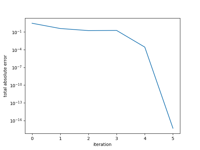
Example 1. Small diagonal matrix.
Example 2: Small random s.p.d. matrix
In our next example, we construct a 5x5 random s.p.d. matrix:
A = rand(5,5)
A = 0.5*(A+A')
A = A + 5*I
with, in this particular instance, eigenvalues
> eigvals(A)

5-element Array{Float64,1}:
 4.46066817714894
 4.979395596044116
 5.2165679905921785
 5.56276039133931
 7.909981699390226
Here the error drops sharply at the 5th iteration, reaching the desired convergence tolerance.
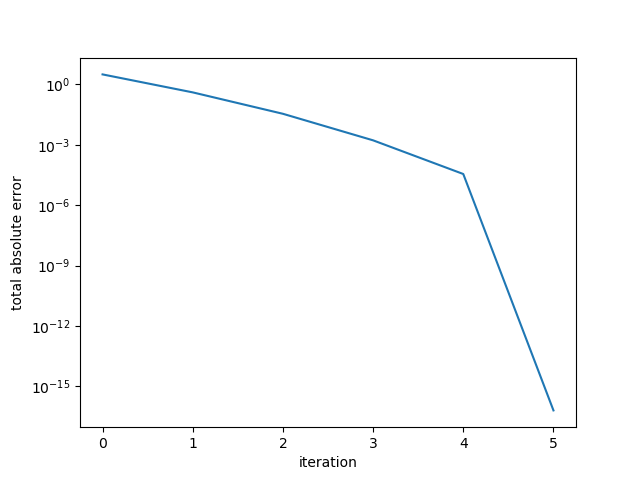
Example 2. Small random s.p.d. matrix.
Example 3: Large random s.p.d. matrix (smaller condition number)
Next, we examine a matrix of dimension 1000, and generate a random s.p.d matrix.
A = rand(N,N)
A = 0.5*(A+A')
A = A + 50*I
Note that in the above snippet, the last line adds a large term to the diagonal, making the matrix “more nonsingular.” The condition number is:
> cond(A)

14.832223763483976
The general rule of thumb is that we lose about 1 digit of accuracy with condition numbers on this order.
The absolute error of the residual is plotted against iteration. Here the algorithm terminated in 11 iterations.
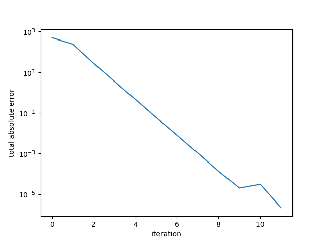
Example 3. Large random s.p.d. matrix, better conditioned.
Example 4: Large random s.p.d. matrix (larger condition number)
Now we examine a matrix again of size 1000 but this time with a smaller multiplier on the diagonal (here we picked the smallest integer value such that the eigenvalues of the resulting matrix were all nonnegative):
A = rand(N,N)
A = 0.5*(A+A')
A = A + 13*I
The condition number is much larger than the previous case, almost at \(10^3\):
> cond(A)

2054.8953570922145
The error plot is below:
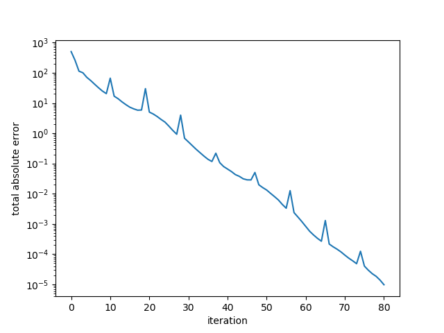
Example 4. Large random s.p.d. matrix, worse conditioned.
Here, the algorithm converged after 80 iterations. A quick check of the “conjugate” vectors shows that the set of vectors is indeed not conjugate.
Code on Github
A Jupyter notebook with all of the code (running Julia v1.0) is available on Github.
References
- Shewchuk. An Introduction to Conjugate Gradient without the Agonizing Pain.
- Nocedal and Wright. Numerical Optimization, Chapter 5.
- Trefethen and Bau. Numerical Linear Algebra, Chapter 6.