Julia v1.0 First Impressions

The Julia Programming Language has finally released version 1.0! I was still using version 0.6 when pretty much suddenly both v0.7 and v1.0 came out within a day apart (thanks JuliaCon).

My LaTeX Setup - vim, Skim, and latexmk

I’ll describe my current LaTeX setup – vim, skim, and latexmk. I currently write notes and papers using LaTeX on a Mac, though in a previous life, my setup on Linux was very similar (i.e., s/macvim/gvim/g and s/skim/zathura/g). I like being able to use my own customized text editor (with my favorite keyboard shortcuts) to edit a raw text file that I can then put under version control. Though I describe things with respect to vim, most of this setup can also achieved with some other text editor, e.g., emacs or sublime.

The basic setup

Text editor: vim

I use the text editor, vim. For writing documents, I often also like using macvim, which is basically vim but with a few extra GUI features, such as scrolling and text selection features.

PDF reader: Skim

For my pdf reader, I use the Skim app. The nice thing about Skim is that it will autoupdate the pdf after you compile the tex and keep the document in the same place. By contrast, Preview will refresh the document and reload it from the beginning of the document, which is quite cumbersome if you’d just edited text on page 5.

Compilation: latexmk + vim keybindings

In vim, I have several keybindings set up in my .vimrc file. Currently, I compile the .tex file using latexmk. Files can be compiled to pdf with the command

latexmk -pdf [file]

In latexmk, you can also automatically recompile the tex when needed, but I prefer to manually compile the tex.

I have the following key bindings in vim:

• control-T compiles the tex to pdf using latexmk
• shift-T opens the pdf in Skim
• shift-C cleans the directory

For instance, the compile keybinding above is done by adding the following line to the .vimrc file

autocmd FileType tex nmap <buffer> <C-T> :!latexmk -pdf %<CR>

These types of key bindings can usually be setup with other text editors as well.

Putting it all together

When I’m writing a document, I’ll often have my text editor full screen on the left and the Skim on the right with the pdf open. After making edits, I’ll press control-T to compile and the pdf will auto-refresh in Skim.

Tools for writing LaTeX documents

There are a few other tools that I use for writing papers (or extensive notes on work) that I’ll list below that save me a lot of time.

Plugins: snippets

In vim, I have several plugins I have in my .vimrc file. For writing papers, I use ()[snippets] extensively. My most used command is typing begin <tab>, which allows me to allows me to autocomplete the parts of LaTeX that I don’t want to spend time typing but use often. For instance, in the TeX below, snippets means I only have to type align* once.

\begin{align*}
    \pi(\theta | x) = \frac{\pi(\theta) p(x | \theta)}
                           {\int \pi(\theta) p(x | \theta) d\theta}
\end{align*}

And should I need to change align* to just align, I only have to edit this in one of the parens instead of in both lines.

To use vim plugins (after installing), you just need to add the github page to your .vimrc file, e.g., for Ultisnips, add the line

Plugin 'SirVer/ultisnips'

and execute :PluginInstall while in command mode in vim.

TeX skeleton

For writing quick notes, I have a TeX skeleton file that always loads when I start a new vim document, i.e., when executing vim notes.tex in the command line, a fully-functional tex skeleton with all the packages I normally use and font styles are automatically loaded. E.g., a version of the following:

\documentclass[11pt]{article}

\usepackage{amsmath, amssymb, amsthm, bbm}
\usepackage{booktabs, fancyhdr, verbatim, graphicx}

\title{title}
\author{Diana Cai}

\begin{document}

\maketitle

\end{document}

subfiles

For longer documents, I use the subfiles package extensively. This allows me to split a document into smaller files, which can then be individually compiled into its own document. Subfiles inherit the packages, etc., that are defined in the main file in which the subfiles are inserted.

The advantage of using subfiles is that you can just edit the subfile you’re currently focusing on, which is much faster than compiling the entire document (especially one with many images and references). This also helps with reducing the number of git conflicts one encounters when collaborating on a document.

macros

I have a set of macros that I commonly use that are imported when I load a .tex document. For writing papers, I’ll include a separate macros.tex file with all of my macro definitions that I reuse often. Some example macros I’ve defined:

• \reals for \mathbb{R}
• \E for \mathbb{E}
• \iid for \stackrel{\mathrm{iid}}{\sim}
• \convas for \stackrel{\mathrm{a.s.}}{\longrightarrow}

Also super convenient if you’re defining a variable that is always bold if, for instance, that variable is a vector.

commenting

My collaborators and I often have a commenting file we use to add various comments (in different colors too!) in the margins, in the text, or highlighting certain regions of the text. An alternative is to use a LaTeX commenting package and then define custom commands controlling how the comments appear in the text.

.vimrc

You can check out my .vimrc file on github to see how I set up keybindings, plugins, and my .tex skeleton file.

Natural gradient descent and mirror descent

In this post, we discuss the natural gradient, which is the direction of steepest descent in a Riemannian manifold [1], and present the main result of Raskutti and Mukherjee (2014) [2], which shows that the mirror descent algorithm is equivalent to natural gradient descent in the dual Riemannian manifold.

Motivation

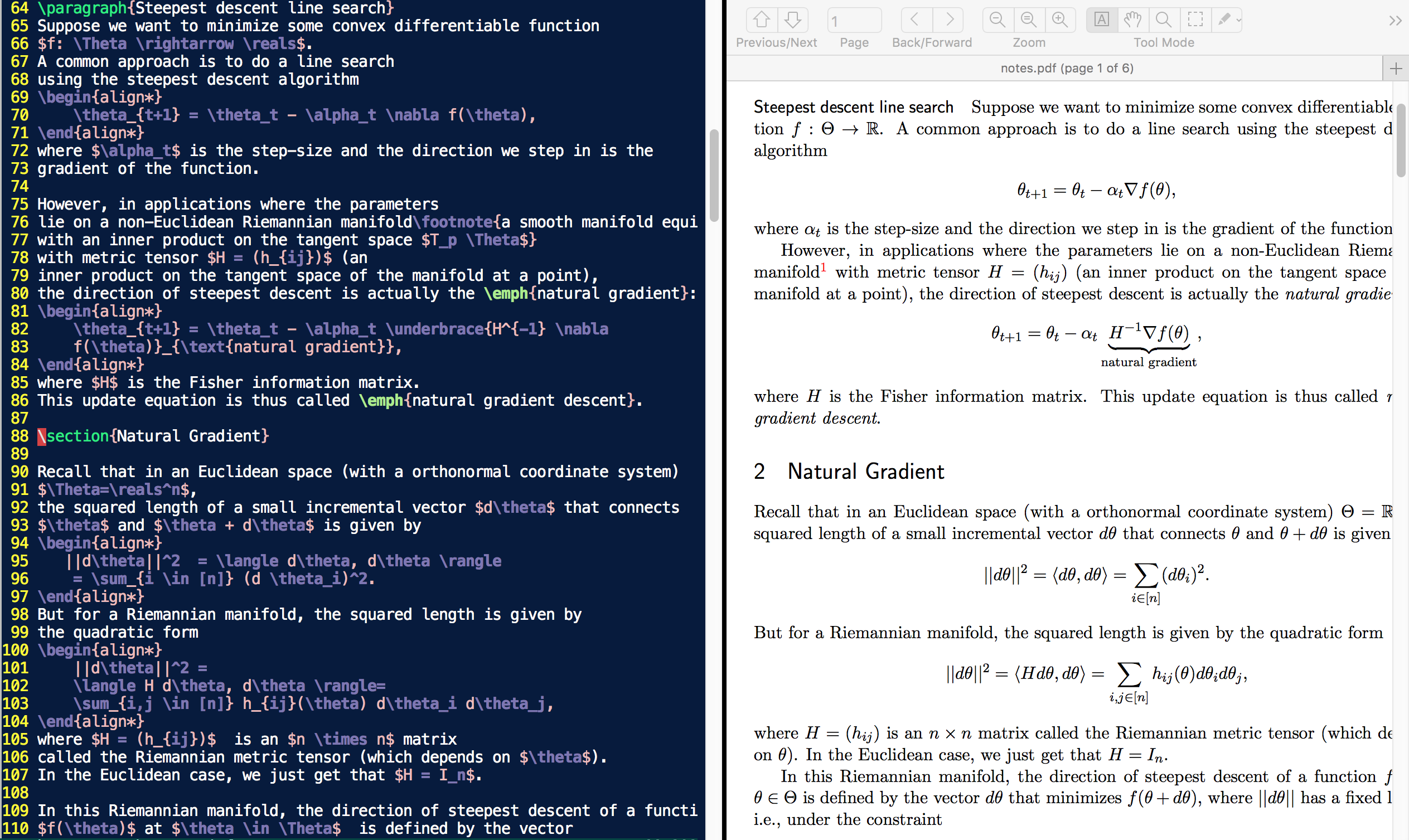
Steepest descent line search

Suppose we want to minimize some convex differentiable function \(f: \Theta \rightarrow {\mathbb{R}}\) . A common approach is to do a line search using the steepest descent algorithm \(\begin{aligned} \theta_{t+1} = \theta_t - \alpha_t \nabla f(\theta),\end{aligned}\) where \(\alpha_t\) is the step-size and the direction we step in is the gradient of the function.

However, in applications where the parameters lie on a non-Euclidean Riemannian manifold¹ with metric tensor \(H = (h_{ij})\) (an inner product on the tangent space of the manifold at a point), the direction of steepest descent is actually the natural gradient:

where \(H\) is the Fisher information matrix for a statistical manifold. This update equation is called natural gradient descent.

Natural Gradients

Recall that in an Euclidean space (with a orthonormal coordinate system) \(\Theta={\mathbb{R}}^n\) , the squared length of a small incremental vector \(d\theta\) that connects \(\theta\) and \(\theta + d\theta\) is given by

But for a Riemannian manifold, the squared length is given by the quadratic form

where \(H = (h_{ij})\) is an \(n \times n\) matrix called the Riemannian metric tensor (which depends on \(\theta\). In the Euclidean case, we just get that \(H = I_n\).

In this Riemannian manifold, the direction of steepest descent of a function \(f(\theta)\) at \(\theta \in \Theta\) is defined by the vector \(d\theta\) that minimizes \(f(\theta + d\theta)\), where \(||d\theta||\) has a fixed length, i.e., under the constraint

Theorem (Amari, 1998) [1]:

The steepest descent direction of \(f(\theta)\) in a Riemannian space is given by

where \(H^{-1} = (h^{ij})\) is the inverse of the metric \(H = (h_{ij})\), and \(\nabla f\) is the conventional gradient:

Proof: Write \(d\theta = \epsilon v\), i.e., we decompose the vector into its magnitude \(\epsilon\) and direction \(v\), and search for the vector \(v\) that decreases the value of the function the most.

Writing the linearized function, we have

subject to the constraint that \(||v||^2 = v^\top H v =1\), i.e., \(v\) is a unit vector representating just the direction.

Setting the derivative with respect to \(v\) of the Lagrangian to 0, i.e.,

so we have that

which is the direction that causes the function’s value to decrease the most. Lastly, plugging \(v\) above into the constraint \(v^\top H v = 1\), we can solve for \(\lambda\).

Thus, the direction of steepest descent is \(H^{-1} \nabla f(\theta)\), i.e., the natural gradient.

Lastly, note that in a Euclidean space, the metric tensor is just the identity matrix, so we get back standard gradient descent.

Mirror descent and Bregman divergence

Mirror descent is a generalization of gradient descent that takes into account non-Euclidean geometry. The mirror descent update equation is

Here \(\Psi: {\mathbb{R}}^p \times {\mathbb{R}}^p \rightarrow {\mathbb{R}}_+\), and when

we get back the standard gradient descent update².

The proximity function \(\Psi\) is commonly chosen to be the Bregman divergence. Let \(G: \Theta \rightarrow {\mathbb{R}}\) be a strictly convex, twice-differentiable function, then the Bregman divergence \(B_G: \Theta \times \Theta \rightarrow {\mathbb{R}}^+\) is:

Equivalence of natural gradient and mirror descent

Bregman divergences and convex duality

The convex conjugate³ of a function \(G\) is defined to be

Now, if \(G\) is a lower semi-continuous function, then we have that \(G\) is the convex conjugate of \(H\). This implies that \(G\) and \(H\) have a dual relationship. If \(G\) is strictly convex and twice differentiable, so is \(H\). Let \(g = \nabla G\) and \(h = \nabla H\). Then \(g = h^{-1}\).

Now let \(\mu = g(\theta) \in \Phi\) be the point at which the supremum for the dual function is attained be the dual coordinate system to \(\theta\). The dual Bregman divergence \(B_H: \Phi \times \Phi \rightarrow {\mathbb{R}}^+\) induced by the strictly convex differentiable function \(H\)

The dual coordinate relationship gives us

• \(B_H(\mu,\mu’) = B_G(h(\mu’), h(\mu))\)

• \(B_G(\theta,\theta’) = B_H(g(\theta’), g(\theta))\)

For exponential families, the function \(G\) is the log partition function⁴. We’ll now work through some examples.

Example: [Normal]

Consider the family \(N(\theta, I_p)\). The log partition function is

and the conjugate function of \(G\) is

since the expression in the supremum is maximized when \(\theta = \mu\) (so we plug this in for \(\theta\) to get the second line). Then we can easily write the Bregman divergence induced by \(G,H\) as

Example: [Poisson]

Now suppose we have the family \(\text{Poisson}(\exp(\theta))\). We have

where we plugged in \(\theta = \log \mu\) above. So the Bregman divergence induced by \(G,H\) is

Bregman divergences and Riemannian manifolds

Now that we have introduced what the Bregman divergence of an exponential family looks like (with respect to the log partition function \(G\) and its dual Bregman divergence with respect to \(H\), where \(H\) is the conjugate of \(G\), we are ready to discuss the respective primal and dual Riemannian manifolds induced by these divergences.

• Primal Riemannian manifold: \((\Theta, \nabla^2 G)\), where \(\nabla^2 G \succ 0\) (since \(G\) is strictly convex and twice differentiable).

• Dual Riemmanian manifold: \(B_H(\theta,\theta’)\) induces the Riemannian manifold \((\Phi, \nabla^2 H)\), where \(\Phi = {\mu: g(\theta) = \mu, \theta \in \Theta}\), i.e., the image of \(\Theta\) under the continuous map \(g = \nabla G\).

Theorem (Raskutti and Mukherjee, 2014) [2]:

The mirror descent step with Bregman divergence defined by \(G\) applied to the function \(f\) in the space \(\Theta\) is equivalent to the natural gradient step along the dual Riemannian manifold \((\Phi, \nabla^2 H)\).

(Proof Sketch):

Step 1: Rewrite the mirror descent update in terms of the dual Riemannian manifold coordinates \(\mu \in \Phi\):

since minimizing by differentiation and the dual coordinates relationship gives us

Step 2: Apply the chain rule:

and plugging this in to the update above, we get

which corresponds to the natural gradient step.

High-level summary:

The main result of [2] is that the mirror descent update with Bregman divergence is equivalent to the natural gradient step along the dual Riemannian manifold.

What does this mean? For natural gradient descent we know that

• the natural gradient is the direction of steepest descent along a Riemannian manifold, and

• it is Fisher efficient for parameter estimation (achieves the CRLB, i.e., the variance of any unbiased estimator is at least as high as the inverse Fisher information),

but neither of these things are known for mirror descent.

The paper also outlines potential algorithmic benefits: natural gradient descent is a second-order method, since it requires the computation of an inverse Hessian, while the mirror descent algorithm is a first-order method and only involves gradients.

References

1. Amari. Natural gradient works efficiently in learning. 1998

2. Raskutti and Mukherjee. The information geometry of mirror descent. 2014.

Footnotes

The Johnson-Lindenstrauss Lemma

The so-called “curse of dimensionality” reflects the idea that many methods are more difficult in higher-dimensions. This difficulty may be due a number of issues that become more complicated in higher-dimensions: e.g., NP-hardness, sample complexity, or algorithmic efficiency. Thus, for such problems, the data are often first transformed using some dimensionality reduction technique before applying the method of choice. In this post, we discuss a result in high-dimensional geometry regarding how much one can reduce the dimension while still preserving \(\ell_2\) distances.

Johnson-Lindenstrauss Lemma

Given \(N\) points \(z_1,z_2,\ldots,z_N \in \mathbb{R}^d\), we want to find \(N\) points \(u_1,\ldots,u_N \in \mathbb{R}^k\), where \(k \ll d\), such that the distance between points is approximately preserved, i.e., for all \(i,j\), \[ ||z_i - z_j||_2 \leq ||u_i - u_j||_2 \leq (1+\epsilon) ||z_i-z_j||_2, \] where \(||z||_2 := \sqrt{\sum_l |z_{l}|^2}\) is the \(\ell_2\) norm. Thus, we’d like to find some mapping \(f\), where \(u_i = f(z_i)\), that maps the data to a much lower dimension while satisfying the above inequalities.

The Johnson-Lindenstrauss Lemma (JL lemma) tells us that we need dimension \(k = O\left(\frac{\log N}{\epsilon^2}\right)\), and that the mapping \(f\) is a (random) linear mapping. The proof of this lemma is essentially given by constructing \(u_i\) via a random projection, and then showing that for all \(i,j\), the random variable \(||u_i - u_j||\) concentrates around its expectation.

This argument is an example of the probabilistic method, which is a nonconstructive method of proving existence of entities with particular properties: if the probability of getting an entity with the desired property is positive, then this entity must be an element of the sample space and therefore exists.

Proof of the JL lemma

We can randomly choose \(k\) vectors \((x_n)_{n=1}^k\), where each \(x_n \in \mathbb{R}^d\), by choosing each coordinate \(x_{nl}\) of the vector \(x_n\) randomly from the set \[ \left\{\left(\frac{1+\epsilon}{k}\right)^{\frac{1}{2}},-\left(\frac{1+\epsilon}{k}\right)^{\frac{1}{2}}\right\}. \]

Now consider the mapping from \(\mathbb{R}^d \rightarrow \mathbb{R}^k\) defined by the inner products of \(z \in \mathbb{R}^d\) with the \(k\) random vectors: \[z \mapsto (z^\top x_1, \ldots, z^\top x_k)\] So, each vector \(u_i = (z_i^\top x_1,\ldots, z_i^\top x_k)\) is obtained via a random projection. (Alternatively, we can think of the mapping as a random linear transformation given by a random matrix \(A \in \mathbb{R}^{k \times d}\), where the \(k\) vectors form the rows of the matrix, and \(Az_i = u_i\).) The goal is to show that there exists some \(u_1,\ldots,u_k\) that satisfies the above inequalities.

Fixing \(i,j\), define \(u := u_i - u_j\) and \(z := z_i - z_j\), and \(Y_n := \left(\sum_{l=1}^d z_l x_{nl} \right)^2\). Thus, we can write the squared \(\ell_2\) norm of \(u\) as \(\begin{aligned} ||u||_2^2 = ||u_i - u_j||_2^2 &= \sum_{n=1}^k \left( \sum_{l=1}^d z_l x_{nl} \right)^2 = \sum_{n=1}^k Y_n \end{aligned},\) where \(x_{nl}\) refers to the \(l\)th component of the \(n\)th vector.

Now we consider the random variable \(Y_n\) in the sum. The expectation is \[ \mathbb{E}(Y_n) = \frac{1+\epsilon}{k} ||z||_2^2. \] So, the expectation of \(||u||_2^2\) is

It remains to show that \(||u||_2^2\) concentrates around its mean \(\mu\), which we can do using a Chernoff bound. In particular, consider the two cases of \(||u||_2^2 > (1 + \delta) \mu\) and \(||u||_2^2 < (1 - \delta) \mu\). Via a Chernoff bound, the probability of at least one of these two “bad” events occurring is upper bounded by \[ \Pr[\{ ||u||^2 > (1+\delta) \mu)\} \lor \{||u||^2 > (1-\delta) \mu \}] < 2\exp(-c \delta^2 k), \] for some \(c > 0\).

Recall that \(||u|| := ||u_i - u_j||\), and so there are \(\binom{N}{2}\) such random variables. Now choosing \(\delta = \frac{\epsilon}{2}\), the probability that any of these random variables is outside of \((1 \pm \frac{\epsilon}{2})\) of their expected value is bounded by

which follows from a union bound.

Choosing \(k > \frac{8(\log N + \log c)}{\epsilon^2}\) ensures that with all \(\binom{N}{2}\) variables are within \((1 \pm \frac{\epsilon}{2})\) of their expectations, i.e., \((1+\epsilon) ||z||_2^2\). Thus, rewriting this, we have that for all \(i,j\),

which then implies the desired result:

References

1. Arora and Kothari. High Dimensional Geometry, Curse of Dimensionality, Dimension Reduction.
2. Dasgupta and Gupta. An Elementary Proof of Theorem of Johnson and Lindenstrauss.
3. Nelson. Dimensionality Reduction Notes Part 1 Part 2

References on Bayesian nonparametrics

Last updated: 11/15/17

This post is a collection of references for Bayesian nonparametrics that I’ve found helpful or wish that I had known about earlier. For many of these topics, some of the best references are lecture notes, tutorials, and lecture videos. For general references, I’ve prioritized listing newer references with a more updated or comprehensive treatment of the topics. Many references are missing, and so I’ll continue to update this over time.

Nonparametric Bayes: an introduction

These are references for people who have little to no exposure to the area, and want to learn more. Tutorials and lecture videos offer a great way to get up to speed on some of the more-established models, methods, and results.

1. Teh (and others). Nonparametric Bayes tutorials.

   This webpage lists a number of review articles and lecture videos that as an introduction to the topic. The main focus is on Dirichlet processes, but a few tutorials cover other topics: e.g., Indian buffet processes, fragmentation-coagulation processes.

2. Broderick. Nonparametric Bayesian Methods: Models, Algorithms, and Applications. 2017. See also joint tutorial with Michael Jordan at the Simon’s Institute.

   An introduction to Dirichlet processes and the Chinese restaurant process, and nonparametric mixture models. Also comes with R code for generating from and sampling (inference) in these models.

3. Wasserman and Lafferty. Nonparametric Bayesian Methods. 2010.

   This gives an overview of Dirichlet processes and Gaussian processes and places these methods in the context of popular frequentist nonparametric estimation methods for, e.g., CDF and density estimation, regression function estimation.

Theory and foundations

It turns out there’s a lot of theory and foundational topics.

1. Orbanz. Lecture notes on Bayesian nonparametrics. 2014.

   A great introduction to foundations of Bayesian nonparametrics, and provides many references for those who want a more in-depth understanding of topics. E.g.: random measures, clustering and feature modeling, Gaussian processes, exchangeability, posterior distributions.

2. Ghosal and van der Vaart. Fundamentals of Bayesian Nonparametric Inference. Cambridge Series in Statistical and Probabilistic Mathematics, 2017. contents

   The most recent textbook on Bayesian nonparametrics, focusing on topics such as random measures, consistency, contraction rates, and also covers topics such as Gaussian processes, Dirichlet processes, beta processes.

3. Kleijn, van der Vaart, van Zanten. Lectures on Nonparametric Bayesian Statistics. 2012.

   Lecture notes with some similar topics as (and partly based on) the Ghosal and van der Vaart textbook, including a comprehensive treatment of posterior consistency.

Specific topics

1. Kingman. Poisson processes. Oxford Studies in Probability, 1993.

   Everything you wanted to know about Poisson processes. (See Orbanz lecture notes above for more references on even more topics on general point process theory.)

2. Pitman. Combinatorial stochastic processes. 2002.

3. Aldous. Exchangeability and related topics. 1985.

4. Orbanz and Roy. Bayesian Models of Graphs, Arrays and Other Exchangeable Random Structures. IEEE TPAMI, 2015.

5. Jordan. Hierarchical models, nested models, and completely random measures. 2013.

6. Broderick, Jordan, Pitman. Cluster and feature modeling from combinatorial stochastic processes. 2013.

Background: probability

Having basic familiarity with measure-theoretic probability is fairly important for understanding many of the ideas in this section. Many of the introductory references aim to avoid measure theory (especially for the discrete models), but even this is not always the case, so it is helpful to have as much exposure as possible.

1. Hoff. Measure and probability. Lecture notes. 2013. pdf

   Gives an overview of the basics of measure-theoretic probability, which are often assumed in many of the above/below references.

2. Williams. Probability with martingales. Cambridge Mathematical Textbooks, 1991.

3. Cinlar. Probability and stochastics. Springer Graduate Texts in Mathematics. 2011.

Models and inference algorithms

There are too many papers on nonparametric Bayesian models and inference methods. Below, I’ll list a few “classic” ones, and continue to add more over time. The above tutorials contain many more references.

Dirichlet processes: mixture models and admixtures

Dirichlet process mixture model

1. Neal. Markov Chain sampling methods for Dirichlet process mixture models. Journal of Computational and Graphical Statistics, 2000. pdf

2. Blei and Jordan. Variational inference for Dirichlet process mixtures. Bayesian Analysis, 2006. pdf

Hierarchical Dirichlet process

1. Teh, Jordan, Beal, Blei. Hierarchical Dirichlet processes. Journal of the American Statistical Association, 2006. pdf

2. Hoffman, Blei, Wang, Paisley. Stochastic variational inference. Journal of Machine Learning Research, 2013. pdf

Nested Dirichlet process & Chinese restaurant process

1. Rodriguez, Dunson, Gelfand. The Nested Dirichlet process. Journal of the American Statistical Association, 2008. pdf

2. Blei, Griffiths, Jordan. The nested Chinese restaurant process and Bayesian nonparametric inference of topic hierarchies. Journal of the ACM, 2010. pdf

3. Paisley, Wang, Blei, Jordan. Nested hierarchical Dirichlet processes. IEEE TPAMI, 2015. pdf

Mixtures of Dirichlet processes

1. Antoniak. Mixture of Dirichlet processes with applications to Bayesian nonparametrics. Annals of Statistics, 1974. pdf

Additional inference methods

1. Ishwaran and James. Gibbs sampling methods for stick-breaking priors. Journal of the American Statistical Association, 2001. pdf

2. MacEachern. Estimating normal means with a conjugate style dirichlet process prior. Communications in Statistics - Simulation and Computation, 1994. pdf

3. Escobar and West. Bayesian density estimation and inference using mixtures. Journal of the American Statististical Association, 1995. pdf

Indian buffet processes and latent feature models

1. Griffiths and Ghahramani. The Indian buffet process: an introduction and review. Journal of Machine Learning Research, 2011. pdf

2. Thibaux and Jordan. Hierarchical beta processes and the Indian Buffet process. AISTATS, 2007. pdf | longer