05 Nov 2017 by Diana Cai
In this post, we will discuss a few simple algorithms for online decision making with expert
advice. In particular, this setting assumes no prior distribution on the set of
outcomes, but we use hindsight to improve future decisions. The algorithms discussed include a simple deterministic and randomized majority weighted decision algorithm.
Lastly, we discuss a randomized algorithm called the multiplicative weights algorithm. This
algorithm has been discovered in a number of fields, and is the basis of many
popular algorithms, such as the Ada Boost algorithm in machine learning and
game-playing algorithms in economics.
This post mostly follows [1] and [2], which contain much more detail on this subject.
In particular, we will omit proofs and refer to these references for the details.
Overview
Consider a setting with \(T < \infty\) rounds. During each round, you get a finite set of actions you can take, e.g.,
\(\mathcal{A} = \{0,1\}\), and associated with each action is some cost
associated with it, that is revealed after taking the action. We would like to
design a policy that minimizes our cost (or maximizes the reward).
For example: consider the scenario of predicting whether or not a single stock’s price
will go up or down. Thus, each round is a day, and the action we take is binary,
corresponding to up/down. At the end of the day, we observe the final price of
the stock: if we make a correct prediction, we lose nothing, but if we make an
incorrect prediction, we lose 1 dollar.
We will consider the setting of total uncertainty, where we a priori have
no knowledge of the distribution on the set of outcomes, e.g., due to lack of
computational resources or data.
We will consider a few algorithms based on knowledge of \(n\) experts.
Predictions with expert advice
Consider again the example of predicting a stock’s price, whose movement can be arbitrary
or adversarial (which comes up, in practice, in a variety of other settings).
But, we get to view the predictions of \(n\) experts (who may or may not be good
at predicting and could even be correlated in some manner).
We would like to design an algorithm that limiting the total cost – i.e., bad predictions – by
limiting it to be about the same as the best expert. Because we do not know who
the best expert is until the end, we need some way of maintaining and updating
our belief of the best expert so that we can make some prediction in each round.
Predicting with the majority
Deterministic algorithm
The simplest algorithm is to just predict according to the majority prediction
of the experts: if most experts predict the price will go up, we will also
predict the price will go up. But what happens if the majority is wrong every
single day? Then, we will lose money every day.
Instead, we can maintain a weight for each expert \(w_i\), that is initially 1
for all experts, but that we decay every time the expert makes a mistake in the
prediction. Then, our action is to predict according to the weighted majority,
which will downweight the predictions of the bad experts. Thus, the algorithm
will predict, at each round, according to the decision with the highest total
weight of the experts.
Let \(\eta \in (0,1)\) be a parameter such that if the expert makes a mistake,
we will decay their weight by \((1-\eta)\), i.e., for the \(i\)th expert, we have
for the \(t\)th round
\[w_i^{(t+1)} = (1-\eta) \, w_i^{(t)}.\]
Then, after \(T\) steps, if \(m_i^{(T)}\) is the number of mistakes from expert
\(i\), we have following bound on the number of mistakes of our algorithm \(M^{(T)}\):
for all \(i\), we have
\[M^{(T)} \leq 2(1+\eta) \, m_i^{(T)} + 2 \frac{\log n}{\eta}.\]
Note that the best expert will have the fewest number of mistakes \(m_i^{(T)}\),
and that the bound holds for all experts. Thus, the number of mistakes the
algorithm makes is roughly a little less than twice the number of mistakes of
the best expert (only the first term depends on \(T\)).
Randomized algorithm
It turns out we can do even better if we convert the above algorithm to a
randomized algorithm. Here, instead of predicting with the weighted majority,
we will predict with the weighted majority with probability proportional to the
weight. For instance, if the total weight of the experts predicting “up” is
\(\frac{3}{4}\), then instead of predicting up, our algorithm will instead
predict up with probability proportional to \(\frac{3}{4}\).
For this algorithm, we instead have the bound
\[M^{(T)} \leq (1+\eta) \, m_i^{(T)} + 2 \frac{\log n}{\eta},\]
which is a factor of 2 less (in the first term) than the above deterministic
algorithm. Thus, this algorithm will perform roughly on the same order as the
best expert.
Multiplicative weights
Now, we consider a more general setting. Here we will choose one decision in
each round out of \(n\) possible decisions, and each decision will incur a
cost, which is revealed after making the decision. Above, we studied the
special case where each decision corresponds to a choice of an expert, and
the cost \(m_i^{(t)}\) is 1 for a mistake, and 0 otherwise. Here we will instead
consister costs that can be in \([-1,1]\).
A naive strategy would be to pick a decision randomly; the expected penalty is
that of the average decision. But, if a few decisions are better, we can observe
this as the costs are revealed, and upweight those better decisions so that we
can pick them in the future. This motivates the multiplicative weight algorithm,
which has been discovered independently in many fields, e.g., machine learning, optimization, and game theory.
The goal is to design an algorithm that, in the long run, has total expected cost roughly on the
order of the best decision, i.e., \(\min_i \sum_{t=1}^T m_i^{(t)}\).
Again, we will maintain a weighting of the decisions \(w_i^{(t)}\), where all weights initially are set to 1.
At each round \(t=1,\ldots,T\), we have a distribution \(p^{(t)}\) over a
set of decisions
\[
p^{(t)} = \left\{\frac{w_1^{(t)}}{\Phi^{(t)}}, \ldots, \frac{w_n^{(t)}}{\Phi^{(t)}} \right\},
\]
where \(\Phi^{(t)} = \sum_i w_i^{(t)}\) is the normalization term.
For each round \(t=1,\ldots,T\), we iterate the following:
-
Randomly select a decision \(i\) from \(p^{(t)}\) (thus, each decision
is chosen with probability proportional to its weight \(w_i^{(t)}\)).
-
The decision is made, and the cost vector \(m^{(t)}\) is revealed, where
the \(i\)th component correponds to the cost of decision \(i\) (with cost \(m_i^{(t)} \in [-1,1]\)). The costs could be chosen arbitrarily by nature.
-
Update the weights of the costly decisions: for each decision \(i\), set
\[
w_i^{(t+1)} = w_i^{(t)} (1 - \eta \, m_i^{(t)}),
\]
where \(\eta \leq \frac{1}{2}\) is fixed in advance.
Here, the multiplicative term \((1-\eta m_i^{(t)})\) is less than 1 (thus, a
decay) if there is a larger cost, but if the cost is negative, this will increase the weights. A cost of 0 would not change the weight at all.
The expected cost of the algorithm from sampling decision \(i \sim p^{(t)}\) is
\[
E_{i \in p^{(t)}}(m_i^{(t)}) = \langle m^{(t)}, p^{(t)} \rangle,
\]
i.e., the sum of the costs weighted by the probability of sampling each respective decision.
The total expected cost is the sum of the expected cost for each round:
\[
\sum_{t=1}^T \langle m^{(t)}, p^{(t)}\rangle.
\]
We can now consider a bound for this value.
Bound for the expected total cost
Assuming all costs \(m_i^{(t)}\) lie in \([-1,1]\), and that \(\eta \leq 1/2\),
then we have the following bound after \(T\) rounds: for any decision
\(i\),
\[
\sum_{t=1}^T \langle m^{(t)}, p^{(t)}\rangle
\leq
\sum_{t=1}^T m_i^{(t)} + \eta \sum_{t=1}^T |m_i^{(t)}| + \frac{\log n}{\eta}.
\]
References
- Arora. Advanced Algorithms notes.
- Arora, Hazan, Kale. The multiplicative weights update method: a meta
algorithm and its applications.
- Borodin and El Yaniv. Online computation and competitive analysis.
21 Oct 2017 by Diana Cai
For data that have a high signal-to-noise ratio, a nonparametric, adaptive method
might be appropriate. In particular, we may want to fit the data to functions
that are spatially imhomogenous, i.e., the smoothness of the function \(f(x)\) varies a lot with \(x\).
In this post, we will discuss wavelets, which can be used an adaptive nonparametric estimation method.
First, we will introduce some background on function spaces and Fourier transforms, and then we will discuss Haar wavelets, a specific type of wavelet, and how to construct wavelets in general.
This presentation follows Wasserman [2], but I’ve included some additional code and images.
Preliminaries
Function spaces
Let \(L_2(a,b)\) denote the set of functions \(f : [a,b] \rightarrow \mathbb{R}\)
such that
\[ \int_a^b f^2(x) dx < \infty.\]
For our purposes, we will assume \(a=0,b=1\).
The inner product of \(f,g \in L_2(a,b)\) is defined as
\[
\langle f,g \rangle :=
\int_a^b f(x) g(x) dx,
\]
and the norm of \(f\) is defined as
\[
|| f || = \left( \int_a^b f^2(x) dx \right)^{\frac{1}{2}}.
\]
A sequence of functions \(\phi_1,\phi_2,\ldots\) is orthonormal if
\(||\phi_j|| = 1 \) for all \(j\) (i.e., has norm 1), and
\( \int_a^b \phi_i(x) \phi_j(x) dx = 0, \,\, i \neq j\) (i.e., orthogonal).
A complete (i.e., the only function orthogonal to each \(\phi_j\) is the 0
function) and orthonormal set of functions form a basis, i.e., if \(f \in L_2(a,b)\),
then \(f\) can be expanded in the basis in the following way:
\[
f(x) = \sum_{j=1}^\infty \theta_j \phi_j(x),
\]
where \(\theta_j = \int_a^b f(x) \phi_j(x) dx \).
A function \(f = \sum_j \beta_j \phi_j \) is sparse in a basis
\(\phi_1,\phi_2,\ldots\) if most of the \(\beta_j\)’s are 0 or close to 0.
Sparseness can be seen as a generalization of smoothness, i.e., a smooth
function is sparse, but there are also nonsmooth functions that are sparse.
Let \(f^{*}\) denote the Fourier transform of a function \(f\):
\[ f^{*}(t) = \int_{-\infty}^\infty \exp(-ixt) \, f(x) \,dx.\]
We can recover \(f\) at almost all \(x\) using the inverse Fourier
transform:
\[
f(x) = \frac{1}{2\pi} \int_{-\infty}^\infty \exp(ixt) \, f^*(t) \,dt,
\]
assuming that \(f^{*}\) is absolutely integrable.
Throughout our discussion of wavelets, we will use the following notation: given
any function \(f\) and \(j,k \in \mathbb{Z}\), define
\[
f_{jk}(x) = 2^{\frac{j}{2}} \, f(2^j x - k).
\]
Wavelets
We now turn our attention to wavelets, beginning with the simplest type of
wavelet, the Haar wavelet.
Haar wavelet
Haar wavelets are a simple type of wavelet given in terms of step-functions.
Specifically, these wavelets are expressed in terms of the the Father and Mother Haar wavelets.
Our goal is to define an orthonormal basis for \(L_2([0,1])\)—to do so,
we need to introduce the Father and Mother wavelets and their shifted and
rescaled sets.
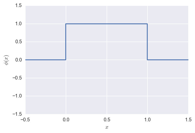
The Father wavelet is defined as:
\[\phi(x) =
\begin{cases}
1 &\text{ if } x \in [0,1] \\
0 &\text{ otherwise } \\
\end{cases}\]
and looks like:
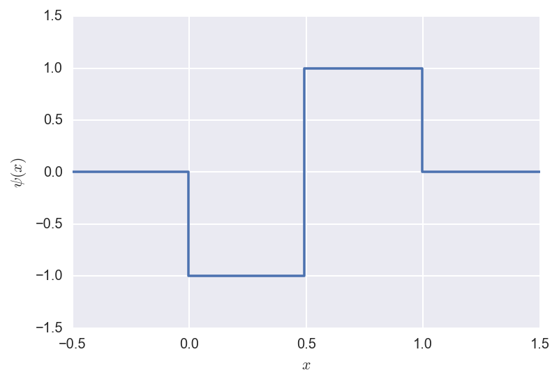
The Mother wavelet is defined as:
\[\psi(x) =
\begin{cases}
-1 &\mathrm{~if~} x \in [0,1/2] \\
1 &\mathrm{~if~} x \in (1/2,1] \\
0 &\mathrm{~otherwise~} \\
\end{cases}\]
and looks like:
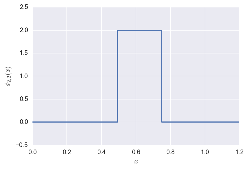
Now we define the wavelets as shifted and rescaled versions of the
Father and Mother wavelets, as above:
\[\phi_{jk}(x) = 2^{j/2} \phi(2^j x - k)\]
and
\[\psi_{jk}(x) = 2^{j/2} \psi(2^j x - k).\]
Below we plot some examples.
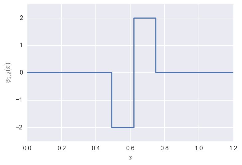
The shifted/rescaled father wavelet \(\phi_{2,2}\) looks like:
The shifted/rescaled mother wavelet \(\psi_{2,2}\) looks like:
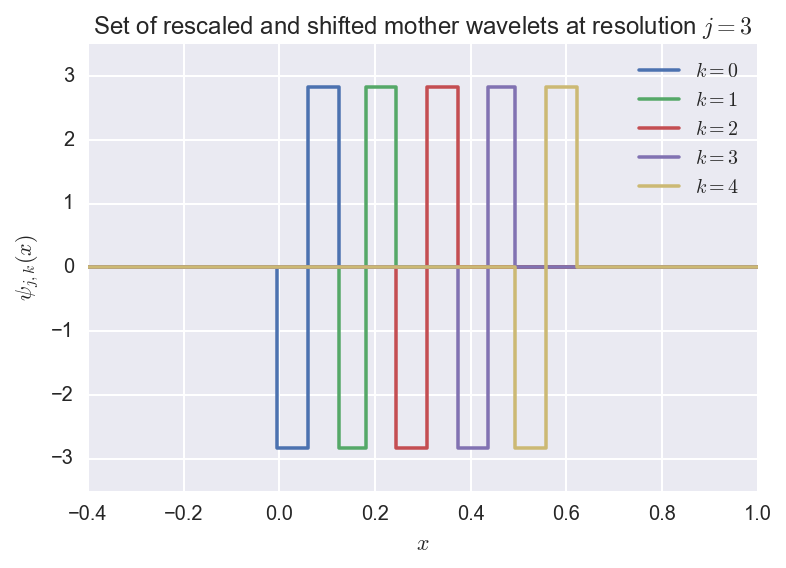
Now we define
the set of rescaled and shifted mother wavelets at resolution $j$
is defined as:
\(W_j = \{\psi_{jk}, k=0,1,\ldots,2^{j-1}\}.\)
We plot an example where \(j=3\):
The next theorem defines gives an orthonormal basis for \(L_2(0,1)\) in terms of
the introduced sets, which allows us to write any function in this space as a
linear combination of the basis elements.
Theorem: The set of functions \(\{\phi, W_0, W_2, W_2,\ldots\}\)
is an orthonormal basis for \(L_2(0,1)\), i.e., the set of real-valued functions on \([0,1]\) where \(\int_0^1 f^2(x) dx < \infty\).
As a result, we can expand any function \(f \in L_2(0,1)\) in this basis:
\[f(x) = \alpha \phi(x) + \sum_{j=0}^{\infty} \sum_{k=0}^{2^j-1}
\beta_{jk} \phi_{jk}(x),\]
where \(\alpha = \int_0^1 \phi(x) dx\) is the scaling coefficient, and
\(\beta_{jk} = \int_0^1 f(x) \psi_{jk}(x) dx\) are the detail coefficients.
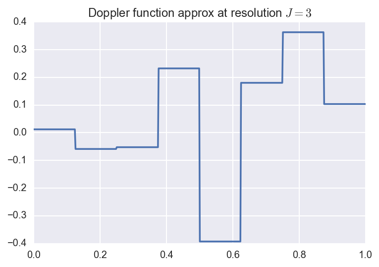
So to approximate a function \(f \in L_2(0,1)\), we can take the finite sum
\[f_J(x) = \alpha \phi(x) + \sum_{j=0}^{J-1} \sum_{k=0}^{2^j-1}
\beta_{jk} \phi_{jk}(x).\]
This is called the resolution \(J\) approximation, and has \(2^J\) terms.
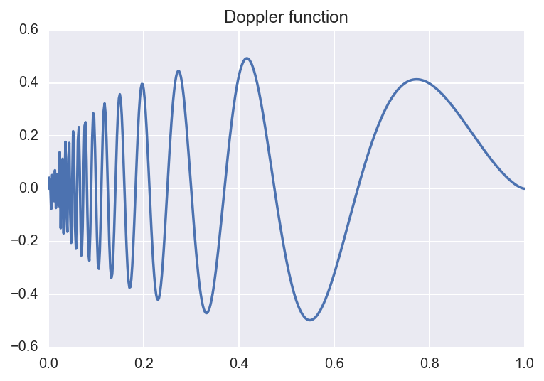
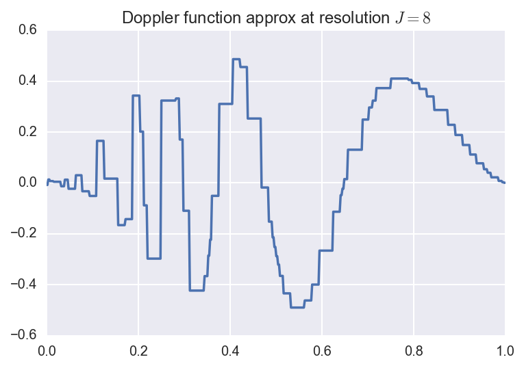
We consider an example below. Suppose we are interested in approximating
the Doppler function:
\[f(x) = \sqrt{x (1-x)} \, \sin(\frac{2.1 \pi}{x + 0.05}).\]
We can approximate this function by considering several resolutions (i.e.,
finite truncations of the wavelet expansion sum).
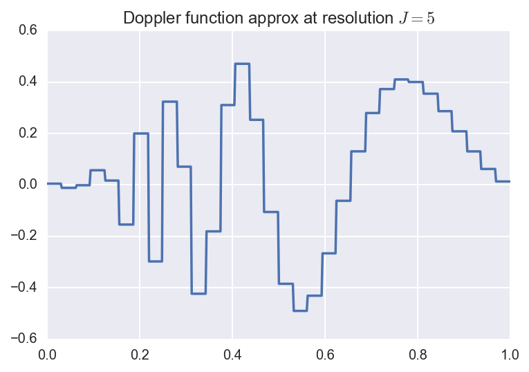
Below, we plot the original function along with the resolution \(J=3,5,8\)
approximations:
Here, the coefficients were computed using numerical quadrature.
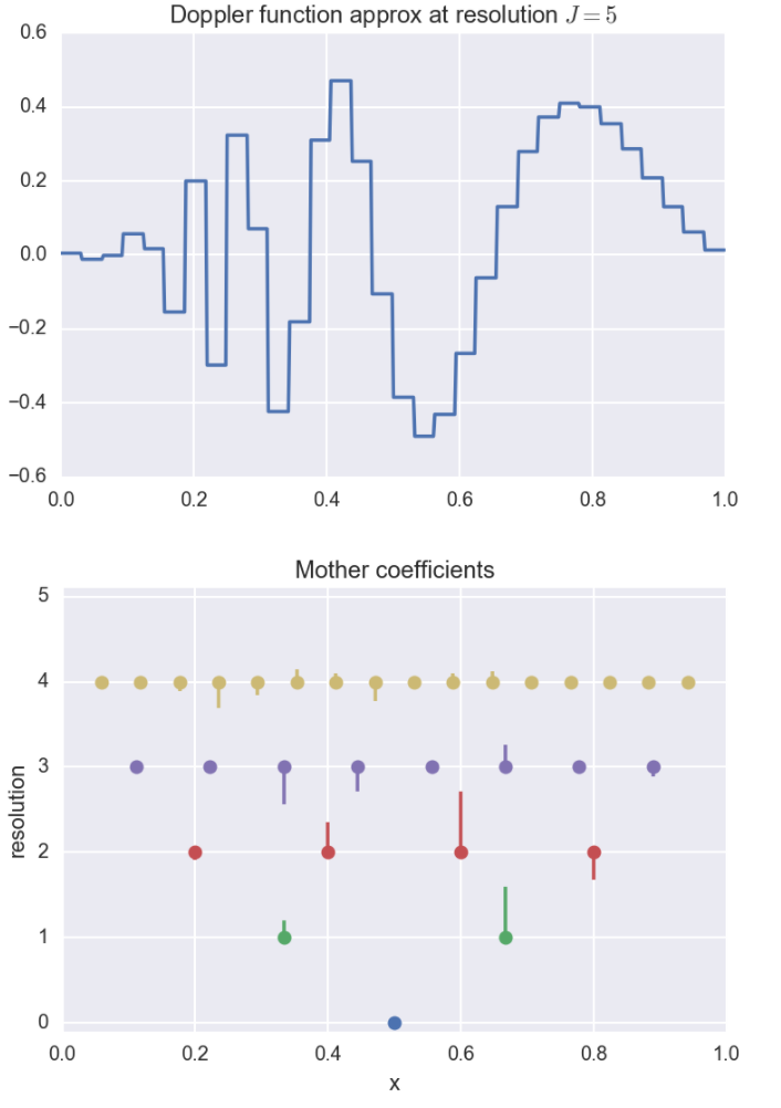
Below, we plot the resolution \(J=5\) approximation along with the coefficients.
The \(y\)-axis represents which resolution or level the coefficient comes from.
The height of the bars are proportional to the size of the coefficients, and the
direction of the bar corresponds to the sign of the coefficient.
For instance, for certain applications, the \(x\)-axis could be represent time, and the resolutions
could then be interpreted as sub-intervals of time.
Constructing smooth wavelets
Haar wavelets are simple to describe and are localized, i.e., the mass is
concentrated in one area. We can express these same ideas for more
general functions, which can give us approximations that are smooth and localized.
Intuitively, it is useful to consider these specific concepts in terms of Haar
wavelets, and to know that we can use these ideas for more general functions \(\phi\) in the following way.
Given any function \(\phi\), we can define the subspaces of \(L_2(\mathbb{R})\) as follows:
\[\begin{align}
V_0 &= \left\{ \,f \,\,\bigl|\,\, f(x) = \sum_{k \in \mathbb{Z}} c_k \,\phi(x - k), \sum_{k \in \mathbb{Z}} c_k^2 \infty \right\} \\
V_1 &= \left\{ \,f(x) = g(2x) \,\,\bigl|\,\, g \in V_0 \right\} \\
V_2 &= \left\{ \,f(x) = g(2x) \,\,\bigl|\,\, g \in V_1 \right\} \\
\vdots
\end{align}\]
Definition: We say that \(\phi\) generates a multiresolution analysis (MRA) of \(\mathbb{R}\) if
\[V_j \subset V_{j+1}, j\geq 0\]
and
\[\bigcup_{j \geq 0} V_j \mathrm{~is~dense~in~} L_2(\mathbb{R}),\]
i.e., for any function \(f \in L_2(\mathbb{R})\), there exists a sequence of functions \(f_1, f_2, \ldots\)
such that each \(f_r \in \bigcup_{j \geq 0} V_j\) and \(||f_r - f|| \rightarrow 0\) as \(r \rightarrow \infty\).
In other words, (…)
Lemma: If \(V_0, V_1, V_2, \ldots\) is an MRA generated by \(\phi\), then
\[\{ \phi_{jk}, k \in \mathbb{Z} \}\]
is an orthonormal basis for \(V_j\).
As an example, we consider the father Haar wavelet as the function \(\phi\).
The the MRA generated by \(\phi\) is given by \(\{\phi, V_0, V_1,\ldots\}\), where
each \(V_j\) is the set of functions \(f \in L_2(\mathbb{R})\) that are
piecewise constant on the interval
\[[k2^{-j}, (k+1) 2^{-j}],\]
for \(k \in \mathbb{Z}\).
Code
Code (Jupyter/iPython notebook) for generating these plots is available on Github.
References
- W. Härdle, G. Kerkyacharian, D. Picard, A. Tsybakov. Wavelets, Approximation, and Statistical Applications.
- L. Wasserman. All of Nonparametric Statistics. Chapter 9.
14 Oct 2017 by Diana Cai
In this post, we’ll review linear systems and linear programming. We’ll then focus on how to use LP relaxations to provide approximate solutions to other (binary integer) problems
that are NP-hard. Much of this post follows these randomized algorithms course notes [1].
Linear programming
One of the most basic ways of thinking of a problem is using linear equations.
It turns out that linear problems are also easy to solve, whereas nonlinear
problems are often hard to solve.
We can express a system of linear equations in matrix form as follows.
Let \(A \in \mathbb{R}^{m \times n}\) be the matrix of coefficients,
\(x \in \mathbb{R}^n \) a vector of variables (that we are interested in),
\(b \in \mathbb{R}^m \) a vector of real numbers.
We can express a system of \(m\) equations and \(n\) variables as the matrix
equation \(Ax=b\).
We can also consider a system of linear inequalities by replacing some of the
equalities with inequalities; i.e., \(Ax \geq b\), where \(\geq\) is a component-wise inequality.
(Throughout this post, we will overload the \(\geq\) symbol and other inequalities to denote both component-wise inequality and scalar inequalities).
The set of solutions is called the feasible region and is a convex polytope.
In the figure below, the edges of the convex polytope are the linear inequalities, and any point in this feasible region satisfies this set of inequalities.
 (Image source:
EMT6680)
(Image source:
EMT6680)
We are often interested in optimizing (e.g., minimizing or maximizing) some
linear function subject to a set of linear inequalities (i.e., constraints).
This is called a linear program (LP) and in its most general form can be expressed
as:
\[ \text{minimize } c^\top x \]
\[ \text{subject to } Ax \geq b, x\geq 0. \]
Here \(c,b\) are known vectors of coefficients, \(A\) is a known matrix of
coeffcients, and \(x\) is the unknown vector of the variables of interest.
(Fun history fact: linear programming was invented in 1939 by the Russian mathematician Leonid
Kantorovich to optimize the organization of industrial production and allocation
of a society’s resources.)
The optimal value of the objective function (that satisfies the constraints) \(x^*\)
will be some vertex/corner/extreme point of the convex feasible region. The simplex algorithm is a
method to enuerate the vertices one by one, decreasing the objective function at
every step.
LP relaxations and approximation algorithms
In a number of problems, the unknown variables are required to be integers,
which defines an integer program. Unlike linear programs, which can be solved
efficiently, integer programs, while being more practical, are NP-hard.
However, what we can do is relax these integer programs so that they are
linear programs, by turning the integer constraints into linear inequalities.
Here we will look at three examples of LP relaxations. The first is an example
that even though we solve the relaxed LP, we still end up with the integer
solution. The other examples require some approximation achieved by rounding.
The assignment problem
We are interested in assigning \(n\) jobs to \(n\) factories, each job having
some cost (raw materials, etc.). Let \(c_{ij}\) dnote the cost of assigning job
\(i\) to factory \(j\), and let \(x_{ij}\) denote the assignment of job \(i\) to
factory \(j\). Thus \(x_{ij}\) is a binary-valued variable and corresponds to a
binary integer program.
To write the relaxed LP program, we turn this binary constraint
into an inequality:
\[ x_{ij} \geq 0 \text{ and } x_{ij} \leq 1,\]
for all \(i,j \in [n] = \{1,\ldots,n\}\). But we also want each job to one
factory and each factory to contain one job.
So, we add the constraint \(\sum_{j=1}^n x_{ij}=1\) for each job
\(i \in [n]\) to guarantee that each job \(i\) is only assigned to one factory,
and the constraint \(\sum_{i=1}^n x_{ij}=1\) for all \(j \in [n]\) to ensure that each factory only gets a single job.
This results in the relaxed LP program
\[\text{minimize } \sum_{ij \in [n]} c_{ij} x_{ij}\]
\[\text{subject to } 0 \leq x_{ij} \leq 1, \quad i,j \in [n] \]
\[\sum_{j=1}^n x_{ij}=1, \quad i \in [n]\]
\[\sum_{i=1}^n x_{ij}=1, \quad j \in [n]\]
This LP results in variables that are all binary and actually solves the
assignment problem.
However, in general, the solution of the LP produces a fractional solution, instead of an integer. Thus, to solve the original integer program, we
can round the fractional solution to get an integer solution.
We now discuss several examples where the LP relaxation gives us a fractional
solution and how we might round these solutions (e.g., deterministically with a
threshold or random rounding).
Approximate rounding solutions
Deterministic rounding
The simplest way to round a fractional solution to a binary one is by picking some threshold, e.g., 1/2, and rounding up or down depending on if variable
is greater than or less than the threshold. We now consider the weighed vertex
cover problem, which is NP-hard, and show that this deterministic rounding
procedure gives us a ``good enough” approximate solution; i.e., with high
probability, we get something within \((1+\epsilon)\) of the true value.
LP relaxation for the weighted vertex cover problem
In the weighted vertex cover problem, we are given a graph \(G = (V,E)\) and
some weight \(w_i \geq 0\) for each vertex \(i\). A vertex
cover is a subset of \(S \subset V\) such that every edge \(e \in E\) has at least one vertex \(v \in S\).
The optimization problem is: find a vertex cover with minimum total weight.
The relaxed LP program is:
\[\text{minimize } f(x) = w^\top x \]
\[\text{subject to } 0 \leq x \leq 1 \]
\[ \quad x_i + x_j \geq 1, \quad\forall \{i,j\} \in E \]
The first line is the objective, i.e., the total weight, where \(x_i\) is a
variable that represents whether vertex \(i\) is in the cover \(S\). The second line
gives the relaxed inequality, and the last line guarantees that we have a vertex
cover, i.e., that for every each edge \(\{i,j\} \in E\), we have at least one vertex that is in the cover (either \(x_i=1\) and/or \(x_j=1\)).
How good is deterministic rounding?
Suppose \(O\) is the optimal value of this program, and let \(V\) be the minimum
weight of the vertex cover problem. We have that \(O \leq V\) since every
binary integer solution is also a fractional solution.
Now apply deterministic rounding to get a new set \(S\), where every vertex
\(i\) with \(x_i \geq \frac{1}{2}\) is in the set, and otherwise not in \(S\).
This produces a vertex cover because for every edge \(\{i,j\} \in E\), we
know that we must satisfy the constraint \(x_i + x_j \geq 1,\) which implies
that \(x_i \geq \frac{1}{2}\) and\or \(x_j \geq \frac{1}{2}\).
Since the optimal value at the solution is
\[O = \sum_{i=1}^n w_i x_i,\]
when we apply the rounding, we only pick the vertices that are greater than
\(\frac{1}{2}\), and so the resulting weight of \(S\) is at most twice the weight of the optimal value
of the LP, i.e., \(2O\). Thus, we have a resulting vertex cover with cost within
a factor of 2 of the optimum cost.
Randomized rounding
Instead of the deterministic thresholding procedure, we could consider a
randomized rounding procedure. One simple randomized rounding procedure is round
the fractional variable \(x_i\) up to 1 with probability \(x_i\) (and down with
probability \(1-x_i\)). The rounded variable therefore has expectation \(x_i\),
and by linearity, the expectation of a linear constraint (i.e., \(c^\top x = d\)) that the fractional
\(x\) satisfies is, in expectation, satisfied by the rounded variable.
We will consider using this randomized rounding procedure for the MAX-2SAT
problem. In this problem, we have \(n\) boolean variables \(x_1,\ldots,x_n\), and a set of clauses of two literals
\(y \vee z\), where each literal is either some \(x_i\) or its negation \(\neg x_i\).
The goal is to find an assignment that maximizes the number of satisfied
clauses \(y \vee z\) (i.e., the clauses is true).
LP relaxation for MAX-2SAT
For this problem, we will form the following LP relaxation. Let \(J\) be a
set of clauses, and \(y_j = (y_{j1}, y_{j2})\) the literals in clause \(j\);
and so \(y_{j1}\) is \(x_i\) if the first literal in clause \(j\) is \(x_i\), and
\(1-x_i\) if it is the negation.
We will define the variable \(z_j\) for each clause \(j\), where
\(\begin{align}
z_j =
\begin{cases}
1 &\text{ if clause } j \text{ satisfied} \\
0 &\text{ otherwise}.
\end{cases}
\end{align}\)
Thus, taking the sum over all \(z_j\) gives us the total number of satisfied clauses,
and thus defines our objective function.
So, we can express this as the relaxed LP
\[\begin{align}
\text{maximize } \sum_{j \in J} & z_j \\
\text{subject to } 1 \geq x &\geq 0 \\
0 \leq z &\leq 1 \\
\mathbf{1}^\top y_j &\geq z_j \qquad \forall j,
\end{align}\]
where \(\mathbf{1}:=[1,1]^\top\).
Here \(x\) and \(z\) are both relaxed to be fractional, and the last line
ensures that the logic of the clauses holds.
How good is randomized rounding?
Now let \(O\) be the optimal value of the this LP, and \(M\) denote the number
of clauses satisfied by the best assignment in MAX-2SAT. We have that
\( M \leq O\).
Now apply randomized rounding to the fractional solution to get the 0/1
assignment. It turns out that the expected number of clauses satisfied is at
least \(\frac{3}{4}\) the optimal value of the LP \(O\).
We can have \(j\) clauses that are either of size 1 or size 2. If the clause
is of size 1, \(x_r\), then the probability it is satisfied is \(x_r\). But we
must have \(x_r \geq z_j\) from the constrainst, so the probability this clause
is satisfied is at least \(\frac{3}{4}z_j\).
Now suppose we have a clause of size 2, e.g., \(x_r \vee x_s\). Note that the
probability of success after randomized rounding is 1 minus the product of if both are 0, i.e.,
\[1 - (1-x_r)(1-x_s) = x_s + x_r - x_r x_s,\]
but since we know from the constraint that
\[z_j \leq x_r + x_s, \]
we can write that the probability of success is at least
\(\begin{align}
x_s + x_r - x_r x_s &\geq x_r + x_s - \frac{1}{4}(x_r + x_s)^2 \\
&\geq z_j - \frac{1}{4}z_j^2 \geq \frac{3}{4} z_j.
\end{align}\)
So, since all clauses individually are satisfied with probability at least
\(\frac{3}{4}z_j\), by linearity of expectation, the expected number of clauses
satisfied is at least \(\frac{3}{4} O\).
Summary
Here we have discussed approximate solutions to integer programs via LP relaxations and two simple rounding schemes. Other problems likely
require more complicated rounding schemes. Here we discussed two problems where
simple deterministic and random rounding give easy to analyze approximate solutions are are
within a constant factor of the solution. Many more rounding schemes and algorithms
can be found in Williamson and Shmoys (2010) [2].
Resources
-
Arora, Kothari, Weinberg (2017). Advanced Algorithm Design Notes
-
Williamson and Shmoys (2010).
Design of Approximation Algorithms
29 Dec 2014 by Diana Cai
Previously, we discussed universal hash families. In this post, we discuss a method of using a 2-universal hash family along with a
Las Vegas algorithm to allow for perfect hashing, where the time required to find an item in a hash table is constant.
A dictionary is a data structure used to maintain a set \(S\) under insertion and deletion of elements, or keys, from some universe \(U\). Dictionaries are typically implemented efficiently using hash tables.
Perfect Hashing
Perfect hashing is a method for storing a static dictionary, i.e. the items are permanently stored in the table, which only needs to support search queries. A hash function \(h: U \rightarrow V\) is called perfect for a set \(S \subset U\) if \(h\) does not cause any collisions among the keys of the set \(S\).
Let \(h\) be chosen uniformly from a 2-universal family of hash functions. Let \(V\) be the range \([0,n-1]\). Then for any set \(S \subset U\) of size \(m\), if the number of items in the universe \(n\) is at least the size of the number of bins squared, \(m^2\), the hash function is perfect with probability at least \(\frac{1}{2}\).
In practice, when \(n \geq m^2\), we can use a Las Vegas algorithm, where we randomly draw hash functions from the 2-universal family until we find one with no collisions, where on average, we only need to try two hash functions. However, this method requires on average \(m^2\) bins.
We can improve the space requirement to having the worst case be \(O(m)\) bins as follows. First, we pick a hash function \(h_1\) uniformly at random from a 2-universal family and hash items in the set using it, resulting in some collisions. We choose the first hash function with a Las Vegas algorithm, trying hash functions until we have at most \(m\) collisions. For each bin with \(k > 1\) items in it (ones with collisions), we can, as before, use \(k^2\) space to achieve no collisions with a second hash function \(h_2\) from a 2-universal family. As before, we use a Las Vegas algorithm to choose the second hash function such that there are no collisions.
Sources:
Mitzenmacher and Upfal. Probability and computing: Randomized algorithms and probabilistic analysis. Cambridge University Press, 2005.
Motwani and Raghavan. Randomized algorithms. Chapman & Hall/CRC, 2010.
06 Sep 2014 by Diana Cai
Hashing is a general method of reducing the size of a set by reindexing the elements into \(n\) bins. This is done using a hash function, which maps some set \( U \) into a range \([0, n-1]\). When designing a hash function, we are interested in something that maps elements into a bin in a way that appears random.
Hashing is used frequently in various randomized algorithms. We now introduce \(k\)-wise independence, which gives a limited notion of independence and discuss it in the context of hashing to construct universal families of hash functions, which give space- and time-efficient data structures.
In future posts, we will discuss various randomized algorithms which use hashing and universal hash families to design efficient and practical approximation algorithms.
Pairwise Independence
\(k\)-wise independence is a useful notion of independence and is more limited than mutual independence, which means that given a set of a random variables or events, any subset of them are independent. In contrast, \(k\)-wise independence says that any subset of random variables that is smaller than
\(k\) is independent, i.e., a set of random variables
\( X_1, X_2, \ldots, X_N \)
is \(k\)-wise independent if, for any subset \(I \subset \{1,\ldots,N\}\) with \(|I| \leq k\) and for any values \(x_i, i\in I \), we have
\[\Pr(\cap_{i\in I} X_i = x_i) = \prod_{i\in I} \Pr(X_i=x_i).\]
In this post, we focus on the case of \(k=2\), or pairwise independence: the random variables \(X_1,X_2,\ldots,X_n\) are pairwise independent if for any pair
\(i,j\) and any values \(a,b\)
\[\Pr(X_i=a, X_j=b) = \Pr(X_i = a) \Pr(X_j=b).\]
Universal Hash Families
When designing hash functions, we want something completely random. However, this model is usually too expensive to compute and store. In practice, we use universal hash families, which have some nice provable properties.
Suppose we have some universe \(U\), which has a cardinality of at least
\(n\), and the set \(V = \{0,1,\ldots,n-1\}\). The family of hash functions
\(\mathcal{H}:U\rightarrow V\) is called \(k\)-universal if for any \(k\)
elements \(x_1,\ldots,x_k\) and hash function \(h\) chosen uniformly
from \(\mathcal{H}\), we have
\[ \Pr(h(x_1)=\ldots=h(x_k)) \leq (n^{k-1})^{-1}.\]
That is, the probability of all \(k\) elements hashing to the same bin is at
most \[\frac{1}{n^{k-1}}.\]
A family of hash functions \(\mathcal{H}:U\rightarrow V\) is called strongly
\(k\)-universal if for any \(k\) elements \(x_1,\ldots,x_k\) and values
\(y_1,\ldots,y_k\), and a randomly chosen hash function \(h\) from
\(\mathcal{H}\), we have
\[\Pr(h(x_1)=y_1,\ldots,h(x_k)=y_k) \leq (n^{k})^{-1}.\]
Strongly \(k\)-universal families are also called \(k\)-wise independent
hash families since \(h(x_1), \ldots, h(x_k)\) are \(k\)-wise independent. Strongly \(k\)-universal families are also \(k\)-universal.
For the rest of this post, we will only consider 2-universal families. When
\(n\) elements are hashed into \(n\) bins using a hash function from a
2-universal hash family, the maximum number of items in a bin is at most
\(\sqrt{2n}\) with probability \(\frac{1}{2}\).
Constructing 2-Universal Families
We now discuss how to generate hash functions from a 2-universal family. Let the
universe \(U = \{0,\ldots,m-1\}\) and let the range be
\(V=\{0,\ldots,n-1\}\), where \(m \geq n\). Choose a prime \(p \geq m\). Consider the hash function
\[h_{ab}(x) = ((ax + b) \mod p)\mod n.\]
The 2-universal hash family is
\[ \mathcal{H} = \left\{h_{a,b} \,|\, 1 \leq a \leq p-1, 0\leq b \leq p-1
\right\}. \]
Thus, to get a 2-universal hash function from this family, we only need to generate \(a\) and \(b\) within the appropriate ranges (note \(a\) cannot be 0).
To generate hash functions from a strongly 2-universal family, we have the family
\[ \mathcal{H} = \left\{h_{a,b} \,|\, 0 \leq a, b \leq p-1 \right\}, \]
where the hash function is given by
\[h_{ab}(x) = (ax + b) \mod p.\]
In future posts, we will describe applications of universal hash families.
Resources
Mitzenmacher, Michael, and Eli Upfal. Probability and computing: Randomized algorithms and probabilistic analysis. Cambridge University Press, 2005.
Motwani, Rajeev, and Prabhakar Raghavan. Randomized algorithms. Chapman & Hall/CRC, 2010.