Schwartz's Theorem and weak posterior consistency
14 Feb 2021Schwartz’s theorem for posterior consistency: In a 1965 paper “On Bayes procedures,” Lorraine Schwartz proved a seminal result on Bayesian consistency of the posterior distribution, which is the idea that as the number of data observations grows, the posterior distribution concentrates on neighborhoods of the true data generating distribution. Under mild regularity conditions on the prior, Schwartz’s theorem leads directly to posterior consistency with respect to the weak topology. In this post, we will state the theorem, discuss the conditions of the theorem, show how the conditions are satisfied for the weak topology as well as a few situations where its easier to satisfy the conditions, and then present a proof of the theorem.
Posterior consistency: an informal picture
Example. Suppose the true data generating distribution of the data (which is unknown to the data analyst) is \(N(0,1)\). The data analyst decides to model the data as i.i.d. from Gaussians of the form \( \mathcal{P} = \{N(\theta, 1): \theta \in \mathbb{R}\} \) and place a Gaussian prior on the unknown parameter \(\theta\). What happens to the posterior distribution as we get more and more data? One should hope that if we have access to an infinite data sample, the posterior should converge towards the “truth.”
Consistency serves a check on some Bayesian analysis. Posterior consistency, which describes the asymptotic behavior when the posterior “concentrates” around the true generating value. In the below plot, we can see that, as we get more data (as visualized by the darker purple curves, or “posterior 1” to “posterior 4”), the posterior mass becomes more peaked around the true value of the parameter (indicated by the black dotted line).
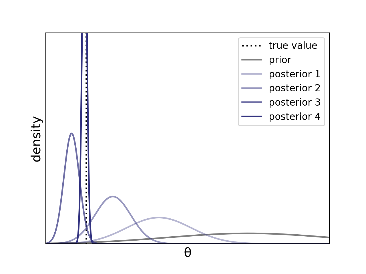
Figure 1. The posterior mass becomes more concentrated around the true parameter value as we get more and more data (i.e., from “posterior 1” to “posterior 4”).
More generally, we can consider some true density \(p_0\) that lives in the model space \(\mathcal{P}\) and a prior on the model space. For instance in the example above, the prior on the parameter \(\theta\) induces a distribution on the space \(\mathcal{P} = \{N(\theta,1): \theta \in \mathbb{R} \} \), and the true density \(p_0 = N(0,1)\) is an element of \(\mathcal{P}\). Roughly, posterior consistency means that as the number of data points \(n \rightarrow \infty\), the posterior distribution (on the model space) will “concentrate” on the true density \(p_0\).
Below is a cartoon informally illustrating posterior concentration around \(p_0\). Here the gray area represents the space of densities given by the model class \(\mathcal{P}\), and the bulk of the posterior mass gets more tightly “peaked” around the true density with more observations.
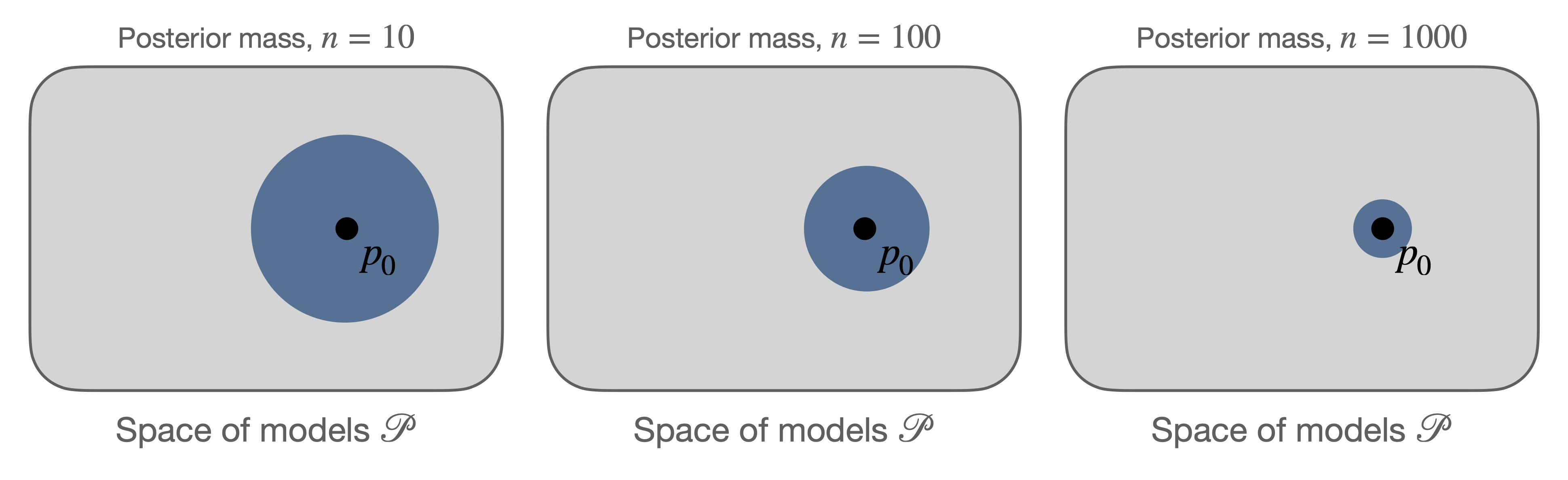
Figure 2. Cartoon illustrating the posterior mass (blue) around the true density \(p_0\) getting more concentrated as the number of data points increases.
In this post, we will make precise what it means for the posterior to “concentrate” and be consistent – here as the number of data points goes to infinity, the posterior mass on densities arbitrarily close to the true density will converge to 1. Then we will present Schwartz’s theorem, one of the primary foundational tools for establishing posterior consistency.
Modeling assumptions
We consider a model class given by a space of densities \(\mathcal{P}\) with respect to a \(\sigma\)-finite measure \(\mu\), and we denote the distribution of a density \(p \in \mathcal{P}\) as \(P\), i.e., \(p = \frac{dP}{d\mu}\). Denote the joint distribution of \(n \in \mathbb{N} \cup \{\infty\} \) samples by \(P^{(n)}\).
Let \(\Pi\) be a prior distribution on our space of models \(\mathcal{P}\), consider the following Bayesian model:
\[\begin{align} p &\sim \Pi \\ X_1,\ldots,X_n \,|\, p &\stackrel{i.i.d.}{\sim} p, \end{align}\]where each \(X_i \in \mathbb{X}\). In this post, we assume the model is well-specified and that there is some true density \(p_0 \in \mathcal{P}\) from which the data are generated.
Under certain conditions on the topology of the parameter space, the posterior distribution exists, and furthermore, because we assume that for every distribution \(P\) in our model class, \(P \ll \mu\), we can compute a version of the posterior distribution via the Bayes’s formula (Ghosal and van der Vaart [1, Chapter 1]).
The posterior distribution \(\Pi(\cdot \,|\, X_1,\ldots, X_n)\) can be expressed as: for all measurable subsets \(A \subseteq \mathcal{P} \),
\[\begin{align} \Pi(A \,|\, X_1,\ldots, X_n) = \frac{\int_{A} \prod_{i=1}^n p(X_i) \,d\Pi(p)}{\int_{\mathcal{P}} \prod_{i=1}^n p(X_i) \,d\Pi(p)}. \end{align}\]Posterior consistency
The posterior distribution \(\Pi(\cdot\,|\, X_1,\ldots,X_n)\) is consistent at \(p_0 \in \mathcal{P}\) if for every neighborhood \(U\) of \(p_0\), with \(P_0^{(\infty)}\)-probability 1 (\(P_0^{(\infty)}\)-a.s.),
\[\begin{align} \Pi(U \,|\, X_1,\ldots,X_n) \stackrel{n\rightarrow \infty}{\longrightarrow} 1. \end{align}\]Remark 1. An alternative way to write the statement above is: for every neighborhood \(U\) of \(p_0\),
\[\begin{align} P_0^{(\infty)}\left(\Pi(U \,|\, X_1,\ldots,X_n) \stackrel{n\rightarrow \infty}{\longrightarrow} 1\right) = 1. \end{align}\]Remark 2. We typically consider the case where \(\mathcal{P} \) is a metric space, and so the neighborhoods of interest are balls around \(p_0\), i.e., \(U = \{p \in \mathcal{P}: d(p_0, p) \leq \epsilon\} \). Commonly used metrics \(d\) include a weak metric (e.g., bounded Lipschitz or Prokhorov), a strong metric (e.g., total variation or Hellinger), or – if we’re working with a Euclidean space for the sample space \(\mathbb{X}\) – a Kolmogorov-Smirnov metric. Note that proving consistency with respect to a strong metric is typically more challenging than with respect to a weak metric and requires stronger conditions.
Remark 3. There are alternative definitions of posterior consistency: sometimes the definition is stated in terms of convergence in probability (as opposed to a.s. convergence) or consistency defined explicitly with a specific topology in mind. For this reason, in our definition above, we avoid the use of the terminology “weak” or “strong” consistency, as that terminology has been used for both the type of convergence of the posterior (i.e., convergence in probability vs a.s. convergence [1]) and to refer to the topology (i.e., weak topology vs strong topology [2]).
Implications of consistency
Posterior consistency – which represents convergence of the posterior towards perfect knowledge – has several implications:
-
Frequentist connection: if the posterior is consistent, then (under some additional technical conditions on the metric used for convergence) the posterior mean is consistent.
-
Bayesian connection: two Bayesian with different priors will have “merging opinions” iff posterior consistency holds. Here a merging opinions refers to the two posteriors of the Bayesian getting closer and closer and we observe more data.
Schwartz’s theorem
Theorem (Schwartz). Let \(\Pi\) be a prior on \(\mathcal{P}\). If \(p_0 \in \mathcal{P}\), and suppose the set \(U\) satisfies:
Condition 1 (prior support): \(p_0\) is in the KL support of the prior \(\Pi\): i.e., for all \(\epsilon > 0\),
\[\begin{align} \Pi(\{p : K(p_0, p) \leq \epsilon\}) > 0, \end{align}\]where \(K(p_0, p) := \int p_0 \log\left( \frac{p_0}{p} \right) d\mu\) is the Kullback-Leibler divergence between \(p_0\) and \(p\).
Condition 2 (testing): There exists a uniformly consistent sequence of tests for testing \(H_0: p = p_0\) vs \(H_1: p \in U^c\): that is, there exist \(\phi_n\) such that
\[\begin{align} P_0^{(n)}(\phi_n) := \int \phi_n \, d P_0^{(n)} &\stackrel{n\rightarrow \infty}{\longrightarrow} 0, \\ \sup_{p \in U^c} P^{(n)}(1-\phi_n) = \sup_{p \in U^c} \int (1-\phi_n) \, d P^{(n)} &\stackrel{n\rightarrow \infty}{\longrightarrow} 0, \end{align}\]where \(\phi_n: \mathbb{X}^n \rightarrow [0,1]\) is a test function.
Then the posterior is consistent at \(p_0\), i.e., for every neighborhood \(U\) of \(p_0\),
\[\begin{align} \Pi(U \,|\, X_1,\ldots,X_n) \stackrel{n\rightarrow \infty}{\longrightarrow} 1, \quad P_0^{(\infty)}\text{-a.s.} \end{align}\]Remarks. Before proving the theorem, we first explain the two main conditions of the theorem. The two conditions impose a constraint on the prior distribution’s support and a the model class via a “testing condition,” respectively.
While the original Schwartz result stated above has limited applicability, small extensions of this theorem have led to a powerful set of tools for analyzing Bayesian asymptotics, and these tools often share assumptions of similar form by imposing constraints on the prior and model class.
Condition 1: KL support of the prior
A basic property of the model needed for posterior consistency is that the prior supports the true density \(p_0\). Recall that the first condition is that the true density \(p_0\) is in the KL support of the prior \(\Pi\), which stipulates that for all \(\epsilon > 0\),
\[\begin{align} \Pi(\{p : K(p_0, p) \leq \epsilon\}) > 0. \end{align}\]Let \(K_\epsilon(p_0) := \{p : K(p_0, p) \leq \epsilon\}\) denote an \(\epsilon\)-KL neighborhood around \(p_0\).
Intuitively, the KL condition says that the prior distribution places positive mass on models arbitrarily close to \(p_0\).
Note that this condition does not say anything about how much mass is near \(p_0\) only that there is positive mass near \(p_0\); stronger results for posterior rates of contraction modify this condition by requiring that there is sufficient amount of mass near the true density.
Condition 2: Uniformly consistent sequence of tests
A test function is a measurable mapping \(\phi_n: \mathbb{X}^n \rightarrow [0,1]\), and denote a test statistic by \(\phi_n(X_1,\ldots,X_n)\).
Recall that a uniformly consistent sequence of tests \(\phi_n\) satisfies:
\[\begin{align} P_0^{(n)}(\phi_n) := \int \phi_n \, d P_0^{(n)} &\stackrel{n\rightarrow \infty}{\longrightarrow} 0, \\ \sup_{p \in U^c} P^{(n)}(1-\phi_n) = \sup_{p \in U^c} \int (1-\phi_n) \, d P^{(n)} &\stackrel{n\rightarrow \infty}{\longrightarrow} 0. \end{align}\]Intuitively, the second condition of Schwartz’s theorem is that “the hypothesis \(H_0: p = p_0\) should be testable against complements of neighborhoods of \(p_0\), i.e., \(H_1: p \in U^c\).” The interpretation of the test \(\phi_n\) is that the null hypothesis \(H_0: p = p_0\) is rejected with probability \(\phi_n\). Given the joint distribution \(P^{(n)}\), then the interpretation of \(P^{(n)} \phi_n\) is the probability of rejecting \(H_0\) when the data are sampled from \(P\).
Thus, the first part of the testing condition \( P_0^{(n)} \phi_n \rightarrow 0 \) has the intepretation that the probability of a Type I error for testing \(H_0\) – i.e., the probability of rejecting \(H_0\) when the data are actually sampled from \(P_0\) – vanishes.
The second part of the testing condition says that for any \(P \in U^c\), \( P^{(n)} (1-\phi_n) \rightarrow 0, \) which has the intepretation that the probability of a Type II error – if \(H_0\) is not rejected but \(P \neq P_0\) – vanishes.
Note that due to the difficulty in directly verifying the uniformly consistent test condition, these conditions themselves are generally not directly checked directly. Some equivalent conditions are given in Ghosh and Ramamoorthi [2], Proposition 4.4.1.
We now discuss three well-studied examples where uniformly consistent sequence of tests exist: (1) under the weak topology, (2) when the sample space is countable, and (3) when the parameter space of the model is finite-dimensional.
Example 1: Posterior consistency with respect to the weak topology
Schwartz’s theorem makes it relatively simple to prove posterior consistency with respect to the weak topology on the model space \(\mathcal{P}\): as we’ll describe in this section, the tests needed for the Schwartz condition exist, and so one only needs to verify the KL support condition.
To establish weak posterior consistency, we need to show that for any weak neighborhood \(U\) of \(p_0\),
\[ \Pi(U^c | X_{1:n}) \stackrel{n\rightarrow\infty}{\longrightarrow 0}, \qquad P_0^{(\infty)}\text{-a.s.}, \]
and so we need to verify the testing condition with respect to the complement \(U^c\).
But it turns out we can simplify this condition by verifying the condition for a simpler set. We first explain why it is sufficient to consider the simpler set, and then we verify the Schwartz testing condition.
Breaking down the posterior
A \(\mu\)-weak neighborhood \(U\) of \(p_0\) is a subset of \(\mathcal{P}\) that can be represented by arbitrary unions of basis elements, given by subsets of the form
\[ V = \left\{ p \in \mathcal{P}: \forall i \in \{1,\ldots,k\}, \left| \int g_i p d\mu - \int g_i p_0 d\mu \right| < \epsilon_i \right\}, \]
where for all \(i\), \(g_i\) is a bounded, real-valued, continuous function on \(\mathbb{X}\), \(\epsilon_i > 0\), and \(k \in \mathbb{N}\).
Note that each basis element \(V\) can be expressed as a finite intersection of subbasis elements, or subsets of the form
\[ V_i = \left\{ p \in \mathcal{P}: \left| \int g_i p d\mu - \int g_i p_0 d\mu \right| < \epsilon_i \right\}, \]
which is an intersection between two sets of the form:
\[ A_i = \left\{ p \in \mathcal{P}: \int g_i p d\mu < \int g_i p_0 d\mu + \epsilon_i \right\}. \]
Thus, the sets of the form \(A_i\) also form a subbasis for \(V\), and the complement \(V^c = \bigcup_{i=1}^{2k} A_i^c \) is then a finite union of the complements of the subbasis elements above.
Since \(V \subset U\) by construction, we can decompose the posterior probability of the complement of the weak neighborhood into a sum of probabilities over the complements of the subbasis sets:
\[\begin{align} \Pi(U^c | X_{1:n}) \leq \Pi(V^c | X_{1:n}) \leq \sum_{i=1}^{2k} \Pi(A_i^c | X_{1:n}). \end{align}\]Thus, in order to prove that \(\Pi(U^c | X_{1:n}) \rightarrow 0, (P_0^{(\infty)}\text{-a.s.})\) as \(n \rightarrow \infty\), it suffices to show that the probability of the subbasis set complements vanish almost surely, i.e., for all \(i\), \(\Pi(A_i^c | X_{1:n}) \rightarrow 0\) a.s.
That is, we only have to verify the testing condition on these subbasis sets.
Satisfying the testing condition
As we discussed above, it suffices to prove the Schwartz testing condition holds for sets of the form
\[ A = \left\{ p \in \mathcal{P}: \int g(x) \, p(x) \, d\mu(x) < \int g(x) \, p_0(x) \, d\mu(x) + \epsilon \right\}. \]
Consider the test function
\[ \phi_n(X_1,\ldots,X_n) = I\left\{\frac{1}{n}\sum_{i=1}^n g(X_i) > \int g(x) \, p_0(x) \, d\mu(x) + \epsilon/2 \right\}. \]
Then the expectation of this test function can be bounded via Hoeffding’s inequality: that is, since \(g\) is a bounded function (and w.l.o.g. can be rescaled such that \(0 \leq g \leq 1\)),
\[ P_0^{(n)} \phi_n = P_0^{(n)}\left(\frac{1}{n}\sum_{i=1}^n g(X_i) > \int g(x) \, p_0(x)\, d\mu(x) + \epsilon/2 \right) \leq e^{-n\epsilon^2/2}. \]
Similarly, another application of Hoeffding’s inequality along with the property that for any \(p \in A^c \), \(\int g(x) p(x) d\mu(x) - \int g(x) p_0(x) d\mu(x) > \epsilon\) implies that \[ P^{(n)}(1-\phi_n) \leq P^{(n)}\left(-\frac{1}{n}\sum_{i=1}^n g(X_i) > -\int g(x) \, p(x)\, d\mu(x) + \epsilon/2 \right) \leq e^{-n\epsilon^2/2}. \]
Thus, in order to guarantee weak posterior consistency holds, we only need to verify that the condition that the prior has positive KL support for the true density, as summarized by the corollary below.
Corollary (Schwartz). Let \(\Pi\) be a prior on \(\mathcal{P}\) and suppose \(p_0\) is in the KL support of the prior \(\Pi\). Then the posterior is weakly consistent at \(p_0\), i.e., for every weak neighborhood \(U\) of \(p_0\),
\[\begin{align} \Pi(U \,|\, X_1,\ldots,X_n) \stackrel{n\rightarrow \infty}{\longrightarrow} 1, \quad P_0^{(\infty)}\text{-a.s.} \end{align}\]Example 2: Countable sample spaces
When the sample space \(\mathbb{X}\) is countable, the weak topology is the same as the topology generated by strong metrics, such as the total variation distance. Thus, Schwartz’s theorem leads to strong posterior consistency for discrete spaces, provided that the prior satisfies the KL support condition.
Example 3: Finite-dimensional models
Suppose the elements model class \(\mathcal{P}\) are parameterized by a finite-dimensional parameter: i.e., \(\theta \mapsto p_\theta\), where \(\theta \in \Theta \subseteq \mathbb{R}^d \). If \(\Theta\) is compact and finite-dimensional, the tests needed exist under mild regularity conditions, i.e., identifiability and continuity of the map \(\theta \mapsto p_\theta\); see, e.g., van der Vaart [7] (1998), Lemma 10.6.
Proof of Schwartz’s theorem
First, rewrite the posterior distribution of the complement of the neighborhood \(U\) as:
\[\begin{align} \Pi(U^c \,|\, X_1,\ldots, X_n) &= \frac{\int_{U^c} \prod_{i=1}^n p(X_i) \,d\Pi(p)}{\int_{\mathcal{P}} \prod_{i=1}^n p(X_i) \,d\Pi(p)} \\\\ &= \frac{\int_{U^c} \prod_{i=1}^n \frac{p(X_i)}{p_0(X_i)} \,d\Pi(p)}{\int_{\mathcal{P}} \prod_{i=1}^n \frac{p(X_i)}{p_0(X_i)} \,d\Pi(p)}. \end{align}\]Since the test functions \(\phi_n \in [0,1]\), we can upper bound the posterior from above as
\[\begin{align} \Pi(U^c \,|\, X_1,\ldots, X_n) &\leq \Pi(U^c \,|\, X_1,\ldots, X_n) + \phi_n(1 - \Pi(U^c \,|\, X_1,\ldots, X_n)) \\\\ &= \phi_n + \frac{(1- \phi_n) \int_{U^c} \prod_{i=1}^n \frac{p(X_i)}{p_0(X_i)} \,d\Pi(p)}{\int_{\mathcal{P}} \prod_{i=1}^n \frac{p(X_i)}{p_0(X_i)} \,d\Pi(p)}. \end{align}\]By Markov’s inequality, the assumption \(P_0^{(n)}(\phi_n) \leq e^{-Cn}\) implies that \(\sum_{n\geq 1} P_0^{(n)}(\phi_n > e^{-Cn}) < \infty, \) and so the Borel–Cantelli lemma then implies that \[P_0^{(\infty)}(\phi_n > e^{-Cn} ~\text{occurs for infinitely many}~ n) = 0. \]
Hence, the first term in the sum above \(\phi_n \rightarrow 0\) almost surely under \(P_0^{(\infty)}\) as \(n \rightarrow \infty\).
It remains to show that the second term has the appropriate behavior. The goal is to control the behavior of the numerator and the denominator of the second term of the sum such that (with \(P_0^{(\infty)}\)-probability 1) this ratio converges to 0.
Step 1:
The KL support condition on the prior \(\Pi\) – i.e., for all \(\epsilon > 0\), \(\Pi(K_\epsilon(p_0)) > 0\) – is used to show that for any \(\beta > 0\),
\[\begin{align} \liminf_{n\rightarrow \infty}~ e^{n\beta} \int_p \prod_{i=1}^n \frac{p(X_i)}{p_0(X_i)} \,d\Pi(p) = \infty \quad P_0^{(\infty)}\text{-a.s.} \end{align}\]Proof of Step 1.
(Expand for proof)
First rewrite the expression as an exponential of the log of the product, which allows us to transform this into a sum of logarithms:
\[\begin{align} e^{n\beta} \int_p \exp\left(\log\left(\prod_{i=1}^n \frac{p(X_i)}{p_0(X_i)}\right)\right) \,d\Pi(p) &= e^{n\beta} \int_p \exp\left(-\sum_{i=1}^n\log\left(\frac{p_0(X_i)}{p(X_i)}\right)\right) \,d\Pi(p) \\ &\geq e^{n\beta} \int_{K_\epsilon(p_0)} \exp\left(-\sum_{i=1}^n\log\left(\frac{p_0(X_i)}{p(X_i)}\right)\right) \,d\Pi(p), \end{align}\]where the second line holds because we are restricting the integral to a smaller set \(K_\epsilon(p_0)\).
Fatou’s lemma gives us an inequality between the liminf outside and the liminf inside the integral:
\[\begin{align} \liminf_{n\rightarrow \infty} \, & e^{n\beta} \int_p \exp\left(\log\left(\prod_{i=1}^n \frac{p(X_i)}{p_0(X_i)}\right)\right) \,d\Pi(p) \\ &\geq \liminf_{n\rightarrow \infty} \, e^{n\beta} \int_{K_\epsilon(p_0)} \exp\left(-\sum_{i=1}^n\log\left(\frac{p_0(X_i)}{p(X_i)}\right)\right) \,d\Pi(p), \\ &\geq \int_{K_\epsilon(p_0)} \liminf_{n\rightarrow \infty} \exp\left(n\beta -\sum_{i=1}^n\log\left(\frac{p_0(X_i)}{p(X_i)}\right)\right) \,d\Pi(p), \end{align}\]Now consider the integrand in the line above and its limiting behavior (thus evaluating its liminf). The strong law of large numbers implies that with \(P_0^{(\infty)}\)-probability 1, for all \(p \in K_\epsilon(p_0)\),
\[\begin{align} -\frac{1}{n}\sum_{i=1}^n\log\left(\frac{p_0(X_i)}{p(X_i)}\right) \stackrel{n\rightarrow\infty}{\longrightarrow} - P_0\log\left(\frac{p_0}{p}\right) = -\int \log\left(\frac{p_0(x)}{p(x)}\right) p_0(x) d\mu(x) = - K(p_0, p) \geq -\epsilon. \end{align}\]where the inequality holds since \(p \in K_\epsilon(p_0)\),
This then implies that with \(P_0^{(\infty)}\)-probability 1,
\[\begin{align} \exp\left(n\left[\beta -\frac{1}{n}\sum_{i=1}^n\log\left(\frac{p_0(X_i)}{p(X_i)}\right)\right]\right) \stackrel{n\rightarrow\infty}{\longrightarrow} \infty. \end{align}\]Plugging this into the liminf above and using the KL support condition, i.e., \(\Pi(K_\epsilon(p_0)) > 0\) and applying Fubini’s theorem, we have
\[\begin{align} \liminf_{n\rightarrow \infty} \, & e^{n\beta} \int_p \prod_{i=1}^n \frac{p(X_i)}{p_0(X_i)} \,d\Pi(p) \\ &\geq \int_{K_\epsilon(p_0)} \liminf_{n\rightarrow \infty} \exp\left(n\left[\beta -\frac{1}{n}\sum_{i=1}^n\log\left(\frac{p_0(X_i)}{p(X_i)}\right)\right]\right) \,d\Pi(p) = \infty \quad P_0^{(\infty)}\text{-a.s.}, \end{align}\]and so the conclusion holds.
Step 2:
The existence of a uniformly sequence of tests is used to show that
\[\begin{align} \lim_{n\rightarrow \infty}~ e^{n\beta_0} (1-\phi_n) \int_{U^c} \prod_{i=1}^n \frac{p(X_i)}{p_0(X_i)} \,d\Pi(p) =0 \quad P_0^{(\infty)} \text{-a.s.} \end{align}\]
(Expand for proof)
By Fubini’s theorem, we can exchange the expectation and integral
\[\begin{align} P_0^{(n)}\left((1 - \phi_n) \int_{U^c} \prod_{i=1}^n \frac{p(X_i)}{p_0(X_i)} \,d\Pi(p)\right) &= \int (1 - \phi_n) \int_{U^c} \prod_{i=1}^n \frac{p(X_i)}{p_0(X_i)} \,d\Pi(p) \, dP_0^{(n)} \\ &= \int_{U^c} \int(1 - \phi_n)\prod_{i=1}^n \frac{p(X_i)}{p_0(X_i)} \, dP_0^{(n)} \,d\Pi(p) \\ &= \int_{U^c} \int (1 - \phi_n)\prod_{i=1}^n p(X_i) d\mu \,d\Pi(p) \\ &= \int_{U^c} \int (1 - \phi_n) \, dP^{(n)} \,d\Pi(p) \\ &= \int_{U^c} P^{(n)} (1 - \phi_n) \,d\Pi(p) \\ &\lesssim e^{-Cn}, \end{align}\]where the last line follows from our assumption that for some \(C > 0\),
\[ \sup_{p \in U^c} P^{(n)} (1 - \phi_n) < e^{-Cn}. \]
And so for some \(\beta_0 > 0, C > 0\),
\[\begin{align} P_0^{(n)}\left(e^{n\beta_0} (1 - \phi_n) \int_{U^c} \prod_{i=1}^n \frac{p(X_i)}{p_0(X_i)} \,d\Pi(p)\right) < e^{-n(C - \beta_0)}. \end{align}\]Since Markov’s inequality implies that \(\sum_{n \geq 1} e^{-n(C - \beta_0)} < \infty \) for \(C > \beta_0\), by the Borel–Cantelli lemma, the numerator goes to 0 almost surely.
Finally, choosing \(\beta = \beta_0\), the ratio goes to 0 a.s.
Remarks on Schwartz’s theorem and extensions
As we saw above, the testing condition of Schwartz’s theorem is always satisfied by the weak neighborhoods. Thus, for weak consistency to hold, all one needs to do is to verify the KL support condition on the prior. But for strong consistency with respect to the L1 metric, uniformly consistent tests do not exist (LeCam, 1973 [4]; Barron, 1989 [5]).
However, it is still possible to get strong posterior consistency via an extension of Schwartz’s theorem. Barron (1988) [6] proved a early result on this, and Ghosal and van der Vaart, Theorem 6.17 (2017) [1] presents an extended Schwartz theorem that can be used to recover the classical Schwartz theorem as well as other consistency results based on metric entropy that are useful for proving, e.g., L1 consistency.
In addition, Schwartz’s theorem has been extended to other related models, such as priors that vary with the data, misspecified models, and non i.i.d. models.
References
-
Ghosal and van der Vaart (2017). Fundamentals of Nonparametric Bayesian Inference (Cambridge Series in Statistical and Probabilistic Mathematics). Cambridge: Cambridge University Press.
-
Ghosh and Ramamoorthi (2003). Bayesian Nonparametrics (Springer Series in Statistics). Springer-Verlag New York.
-
Schwartz (1965). On Bayes procedures. Z. Wahrsch. Verw. Gebiete 4, 10–26.
-
LeCam. Convergence of estimates under dimensionality restrictions (1973). Annals of Statistics, 1:38–53.
-
Barron (1989). Uniformly powerful goodness of fit tests. Annals of Statistics, 17(1):107–124.
-
Barron (1988). The exponential convergence of posterior probabilities with implications for Bayes estimators of density functions. Technical Report 7, Dept. Statistics, Univ. Illinois, Champaign.
-
Van der Vaart, A. W. (2000). Asymptotic statistics (Vol. 3). Cambridge university press.