The Extended Schwartz Theorem and strong posterior consistency

Schwartz’s theorem is a classical tool used to derive posterior consistency and is the foundation of many modern results for establishing frequentist consistency of Bayesian methods. As we discuss in our post on the original Schwartz result, the theorem itself had somewhat limited applicability; it was straightforward to use to establish weak consistency, provided the KL support condition on the prior holds, but was generally not enough to guarantee posterior consistency with respect to strong metrics, such as the L1 distance. This is because the uniformly consistent tests do not always exist for other metrics.

But an extension of Schwartz’s original theorem makes it much more broadly applicable. In this post, we review the extended Schwartz theorem, show how it can be used to recover the classical Schwartz theorem, and how it can be used to establish “strong” posterior consistency. For an introduction to posterior consistency and basic definitions, see our post on the original Schwartz result.

Preliminaries and notation

We consider the same i.i.d. modeling setting as in our discussion on classical Schwartz. Let \(\mathcal{P}\) denote our model class, which is a space of densities with respect to a \(\sigma\)-finite measure \(\mu\), where \(p: \mathbb{X} \rightarrow \mathbb{R}\) is a measurable function that is nonnegative and integrates to 1. We denote the distribution of a density \(p \in \mathcal{P}\) as \(P\), i.e., \(p = \frac{dP}{d\mu}\). Denote the joint distribution of \(n \in \mathbb{N} \cup \{\infty\} \) samples by \(P^{(n)}\).

Let \(\Pi\) be a prior distribution on our space of models \(\mathcal{P}\), consider the following Bayesian model:

where each \(X_i \in \mathbb{X}\). In this post, we assume the model is well-specified and that there is some true density \(p_0 \in \mathcal{P}\) from which the data are generated.

Under certain regularity conditions on \(\mathcal{P}\), (a version of) the posterior distribution, \(\Pi(\cdot \,|\, X_1,\ldots, X_n)\), can be expressed via the Bayes’s formula: for all measurable subsets \(A \subseteq \mathcal{P} \),

The Extended Schwartz Theorem

The statement of the theorem in Ghosal and van der Vaart has two parts; here we state the first part below as a theorem – which provides tools for more general results – and the second part as a corollary – which leads to insights directly about posterior consistency. Lastly, we’ll discuss how to prove the classical Schwartz’s theorem using the extended version, and how to get results on strong posterior consistency.

Theorem (Extended Schwartz). Suppose there exists a set \( \mathcal{P}_0 \subseteq \mathcal{P} \) and a number \(c\) with \(\Pi(\mathcal{P}_0) > 0 \) and \(K(p_0; \mathcal{P}_0) \leq c. \) Let \(\mathcal{P}_n \subseteq \mathcal{P}\) be a set that satisfies either condition (a) or condition (b) for some constant \(C > c\):

(a) There exist tests \(\phi_n\) such that

(b) The prior satisfies \(\begin{align} \Pi(\mathcal{P}_n) \leq e^{-Cn}. \end{align}\)

Then

Remarks on theorem statement

The theorem above provides some conditions under which the posterior probability of the set \(\mathcal{P}_n \) goes to 0 with probability 1. At the expense of its greater generality, this version of the theorem may as a result appear more mysterious in its application.

First recall that \(\mathcal{P}\) is the space of densities of our model class. The statement describes behaviors for two general subsets of densities \(\mathcal{P}_0\) and \(\mathcal{P}_n\):

• What are the sets \(\mathcal{P}_0\)? These sets show up in conditions on the prior / KL divergence bound and serve as a prior support condition. E.g, it is applied to KL neighborhoods in the classical Schwartz theorem.

• What are the sets \(\mathcal{P}_n\)? These sets are present in the conditions (a) and (b) as well as in the asymptotic result. The theorem allows us to establish when the posterior probability of a general subset \(\mathcal{P}_n\ \subseteq \mathcal{P} \) is going 0 a.s., rather than a specific subset needed to show consistency (e.g., a neighborhood of \(p_0\)). As we’ll see below, we’ll apply this to show posterior consistency by decomposing the complement of a neighborhood \(U^c\) into a union of two other subsets, and apply this general theorem to each of the other subsets.

Regarding the conditions (a) and (b), note that either (a) or (b) needs to hold to imply the result. First note that condition (b) a special case of condition (a) when \(\phi_n = 0\), but serves as a useful restatement of (a), as we’ll see in the proof of the corollary. Thus, in order to prove \( \Pi(\mathcal{P}_n \,|\, X_{1:n}) \stackrel{n\rightarrow\infty}{\longrightarrow} 0 ~(P_0^{(\infty)}\text{-a.s.}), \) we only need to assume condition (a) holds.

Condition (a). These two conditions should look familiar and close to the classical Schwartz testing conditions. One condition that is commonly used to verify the classical Schwartz theorem is that the sequence of tests have exponentially small error probabilities (Ghosh and Ramamoorthi [2], Proposition 4.4.1): i.e., for some \(C > 0\),

where in the classical Schwartz theorem, \(\mathcal{P}_n = U^c\).

Here \(P_0^{(n)}(\phi_n) \leq e^{-Cn}\) implies, via the Borel-Cantelli lemma, the first part of the condition in the extended Schwartz theorem, i.e., that \(\phi_n \rightarrow 0\) a.s. And in the extended Schwartz theorem, the second part of the condition replaces \(\sup_{p \in U^c} P^{(n)}(1- \phi_n) \leq e^{-Cn}\) with an integral against the prior distribution \(\Pi\) over the set of densities in \(\mathcal{P}_n\).

Condition (b). This condition essentially says that if \(\mathcal{P}_n\) is a set that the prior assigns a small amount of mass to, then asymptotically, the posterior will also assign a small amount of mass to that set.

Proof of theorem

The proof itself follows similar steps to that of the proof of the classical Schwartz theorem; see our post on the classical Schwartz for additional details. We include a sketch below for completeness.

Corollary: posterior consistency

The theorem above implies the following result on posterior consistency, which is more readily compared to the statement of the classical Schwartz theorem.

Corollary (Extended Schwartz). Consider the model

Suppose that \(p_0\) is in the KL support of the prior, i.e., \(p_0 \in \mathrm{KL}(\Pi)\), and that for every neighborhood \(U\) of \(p_0\), there exists a constant \(C > 0\), measurable partitions \(\mathcal{P} = \mathcal{P_{n,1}} \sqcup \mathcal{P_{n,2}}\) and tests \(\phi_n\) such that the following conditions hold:

(i) The test functions satisfy

(ii) The prior satisfies \(\begin{align} \Pi(\mathcal{P}_{n,2}) \leq e^{-Cn}. \end{align}\)

Then the posterior is consistent at \(p_0\): i.e., for every neighborhood \(U\) of \(p_0\),

Remarks on corollary statement

In particular, the conditions are essentially the same as the classical Schwartz theorem, but now we split the space of densities \(\mathcal{P}\) into (1) one part \(\mathcal{P}_{n,1}\) that goes into the testing condition, and (2) another part \(\mathcal{P}_{n,2}\) that has small prior mass and therefore small posterior mass (and so does not need to be tested). In the Bayesian asymptotics literature, the sequence of sets \(\{\mathcal{P}_{n,1}\}\) are often called sieves.

If we take \(\mathcal{P}_{n,1} = \mathcal{P}\) and \(\mathcal{P}_{n,2} = \emptyset\), then the extended Schwartz conditions (i) and (ii) imply that the same testing conditions as classical Schwartz hold, i.e., that the test sequence is uniformly consistent.

Proof of the corollary

The result follows from applying parts (a) and (b) separately from the theorem above.

Strong posterior consistency

In this section, we state a theorem that establishes strong posterior consistency, i.e., posterior consistency with the strong topology; this result is a consequence of applying the extended Schwartz theorem above. Note: the statement of this corollary in Ghosal and van der Vaart (2017) [1] uses the terminology “strongly consistent” to refer to \(P_0\)-a.s. consistency, rather than referring to convergence in the strong topology.

Preliminaries: covering and metric entropy

In order to establish a more direct strong posterior consistency result, the (extended Schwartz) testing condition is replaced with a bound on the complexity of the space, which is measured by a function of the covering number \(N(\epsilon, \mathcal{P}_{n,1}, d)\) with respect to the set \(\mathcal{P}_{n,1} \subseteq \mathcal{P}\). In order to define the covering number, we need to first introduce another definition.

A set \(S\) is called an \(\epsilon\)-net for \(T\) if for every \(t \in T\), there exists \(s \in S\) such that \(d(s,t) < \epsilon\). This means that the set \(T\) is covered by a collection of balls of radius \(\epsilon\) around the points in the set \(S\). The \(\epsilon\)-covering number, denoted by \(N(\epsilon, T, d)\), is the minimum cardinality of an \(\epsilon\)-net.

The quantity \(\log N(\epsilon, T, d)\) is called metric entropy, and a bound on this quantity is a condition that appears in many posterior concentration results.

Strong posterior consistency via extended Schwartz

Again we consider the model \(X_{1:n} \,|\, p \stackrel{i.i.d.}{\sim} p\) and \(p \sim \Pi \). The following theorem leads to posterior consistnecy with respect to any distance \(d\) that is bounded above by the Hellinger distance, e.g., the \(\mathcal{L}_1\) distance.

Theorem (strong consistency). Let \(d\) be a distance that generates convex balls and satisfies \(d(p_0, p) \leq d_H(p_0, p)\) for every \(p\). Suppose that for every \(\epsilon > 0\), there exist partitions \(\mathcal{P} = \mathcal{P}_{n,1} \sqcup \mathcal{P}_{n,2}\) and a constant \(C > 0\) such that, for sufficiently large \(n\),

1. \( \log N(\epsilon, \mathcal{P}_{n,1}, d) \leq n \epsilon^2, \)

2. \( \Pi(\mathcal{P}_{n,2}) \leq e^{-Cn}. \)

Suppose \(p_0 \in \text{KL}_\epsilon(\Pi)\). Then the posterior distribution is consistent at \(p_0\).

References

1. Ghosal and van der Vaart (2017). Fundamentals of Nonparametric Bayesian Inference (Cambridge Series in Statistical and Probabilistic Mathematics). Cambridge: Cambridge University Press.

2. Kleijn, van der Vaart, van Zanten. Lectures on Nonparametric Bayesian Statistics

Schwartz's Theorem and weak posterior consistency

Schwartz’s theorem for posterior consistency: In a 1965 paper “On Bayes procedures,” Lorraine Schwartz proved a seminal result on Bayesian consistency of the posterior distribution, which is the idea that as the number of data observations grows, the posterior distribution concentrates on neighborhoods of the true data generating distribution. Under mild regularity conditions on the prior, Schwartz’s theorem leads directly to posterior consistency with respect to the weak topology. In this post, we will state the theorem, discuss the conditions of the theorem, show how the conditions are satisfied for the weak topology as well as a few situations where its easier to satisfy the conditions, and then present a proof of the theorem.

Posterior consistency: an informal picture

Example. Suppose the true data generating distribution of the data (which is unknown to the data analyst) is \(N(0,1)\). The data analyst decides to model the data as i.i.d. from Gaussians of the form \( \mathcal{P} = \{N(\theta, 1): \theta \in \mathbb{R}\} \) and place a Gaussian prior on the unknown parameter \(\theta\). What happens to the posterior distribution as we get more and more data? One should hope that if we have access to an infinite data sample, the posterior should converge towards the “truth.”

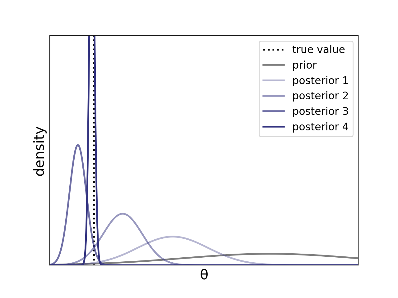
Consistency serves a check on some Bayesian analysis. Posterior consistency, which describes the asymptotic behavior when the posterior “concentrates” around the true generating value. In the below plot, we can see that, as we get more data (as visualized by the darker purple curves, or “posterior 1” to “posterior 4”), the posterior mass becomes more peaked around the true value of the parameter (indicated by the black dotted line).

More generally, we can consider some true density \(p_0\) that lives in the model space \(\mathcal{P}\) and a prior on the model space. For instance in the example above, the prior on the parameter \(\theta\) induces a distribution on the space \(\mathcal{P} = \{N(\theta,1): \theta \in \mathbb{R} \} \), and the true density \(p_0 = N(0,1)\) is an element of \(\mathcal{P}\). Roughly, posterior consistency means that as the number of data points \(n \rightarrow \infty\), the posterior distribution (on the model space) will “concentrate” on the true density \(p_0\).

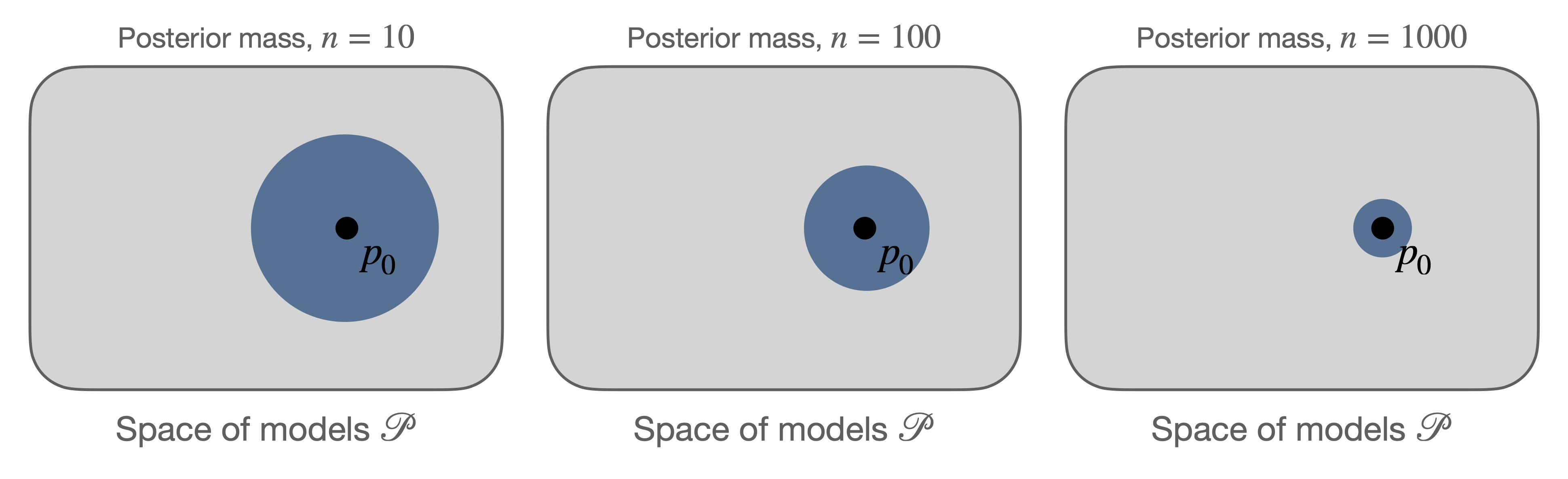
Below is a cartoon informally illustrating posterior concentration around \(p_0\). Here the gray area represents the space of densities given by the model class \(\mathcal{P}\), and the bulk of the posterior mass gets more tightly “peaked” around the true density with more observations.

In this post, we will make precise what it means for the posterior to “concentrate” and be consistent – here as the number of data points goes to infinity, the posterior mass on densities arbitrarily close to the true density will converge to 1. Then we will present Schwartz’s theorem, one of the primary foundational tools for establishing posterior consistency.

Modeling assumptions

We consider a model class given by a space of densities \(\mathcal{P}\) with respect to a \(\sigma\)-finite measure \(\mu\), and we denote the distribution of a density \(p \in \mathcal{P}\) as \(P\), i.e., \(p = \frac{dP}{d\mu}\). Denote the joint distribution of \(n \in \mathbb{N} \cup \{\infty\} \) samples by \(P^{(n)}\).

Let \(\Pi\) be a prior distribution on our space of models \(\mathcal{P}\), consider the following Bayesian model:

where each \(X_i \in \mathbb{X}\). In this post, we assume the model is well-specified and that there is some true density \(p_0 \in \mathcal{P}\) from which the data are generated.

Under certain conditions on the topology of the parameter space, the posterior distribution exists, and furthermore, because we assume that for every distribution \(P\) in our model class, \(P \ll \mu\), we can compute a version of the posterior distribution via the Bayes’s formula (Ghosal and van der Vaart [1, Chapter 1]).

The posterior distribution \(\Pi(\cdot \,|\, X_1,\ldots, X_n)\) can be expressed as: for all measurable subsets \(A \subseteq \mathcal{P} \),

Posterior consistency

The posterior distribution \(\Pi(\cdot\,|\, X_1,\ldots,X_n)\) is consistent at \(p_0 \in \mathcal{P}\) if for every neighborhood \(U\) of \(p_0\), with \(P_0^{(\infty)}\)-probability 1 (\(P_0^{(\infty)}\)-a.s.),

Remark 1. An alternative way to write the statement above is: for every neighborhood \(U\) of \(p_0\),

Remark 2. We typically consider the case where \(\mathcal{P} \) is a metric space, and so the neighborhoods of interest are balls around \(p_0\), i.e., \(U = \{p \in \mathcal{P}: d(p_0, p) \leq \epsilon\} \). Commonly used metrics \(d\) include a weak metric (e.g., bounded Lipschitz or Prokhorov), a strong metric (e.g., total variation or Hellinger), or – if we’re working with a Euclidean space for the sample space \(\mathbb{X}\) – a Kolmogorov-Smirnov metric. Note that proving consistency with respect to a strong metric is typically more challenging than with respect to a weak metric and requires stronger conditions.

Remark 3. There are alternative definitions of posterior consistency: sometimes the definition is stated in terms of convergence in probability (as opposed to a.s. convergence) or consistency defined explicitly with a specific topology in mind. For this reason, in our definition above, we avoid the use of the terminology “weak” or “strong” consistency, as that terminology has been used for both the type of convergence of the posterior (i.e., convergence in probability vs a.s. convergence [1]) and to refer to the topology (i.e., weak topology vs strong topology [2]).

Implications of consistency

Posterior consistency – which represents convergence of the posterior towards perfect knowledge – has several implications:

1. Frequentist connection: if the posterior is consistent, then (under some additional technical conditions on the metric used for convergence) the posterior mean is consistent.

2. Bayesian connection: two Bayesian with different priors will have “merging opinions” iff posterior consistency holds. Here a merging opinions refers to the two posteriors of the Bayesian getting closer and closer and we observe more data.

Schwartz’s theorem

Theorem (Schwartz). Let \(\Pi\) be a prior on \(\mathcal{P}\). If \(p_0 \in \mathcal{P}\), and suppose the set \(U\) satisfies:

Condition 1 (prior support): \(p_0\) is in the KL support of the prior \(\Pi\): i.e., for all \(\epsilon > 0\),

\[\begin{align} \Pi(\{p : K(p_0, p) \leq \epsilon\}) > 0, \end{align}\]

where \(K(p_0, p) := \int p_0 \log\left( \frac{p_0}{p} \right) d\mu\) is the Kullback-Leibler divergence between \(p_0\) and \(p\).

Condition 2 (testing): There exists a uniformly consistent sequence of tests for testing \(H_0: p = p_0\) vs \(H_1: p \in U^c\): that is, there exist \(\phi_n\) such that

\[\begin{align} P_0^{(n)}(\phi_n) := \int \phi_n \, d P_0^{(n)} &\stackrel{n\rightarrow \infty}{\longrightarrow} 0, \\ \sup_{p \in U^c} P^{(n)}(1-\phi_n) = \sup_{p \in U^c} \int (1-\phi_n) \, d P^{(n)} &\stackrel{n\rightarrow \infty}{\longrightarrow} 0, \end{align}\]

where \(\phi_n: \mathbb{X}^n \rightarrow [0,1]\) is a test function.

Then the posterior is consistent at \(p_0\), i.e., for every neighborhood \(U\) of \(p_0\),

Remarks. Before proving the theorem, we first explain the two main conditions of the theorem. The two conditions impose a constraint on the prior distribution’s support and a the model class via a “testing condition,” respectively.

While the original Schwartz result stated above has limited applicability, small extensions of this theorem have led to a powerful set of tools for analyzing Bayesian asymptotics, and these tools often share assumptions of similar form by imposing constraints on the prior and model class.

Condition 1: KL support of the prior

A basic property of the model needed for posterior consistency is that the prior supports the true density \(p_0\). Recall that the first condition is that the true density \(p_0\) is in the KL support of the prior \(\Pi\), which stipulates that for all \(\epsilon > 0\),

Let \(K_\epsilon(p_0) := \{p : K(p_0, p) \leq \epsilon\}\) denote an \(\epsilon\)-KL neighborhood around \(p_0\).

Intuitively, the KL condition says that the prior distribution places positive mass on models arbitrarily close to \(p_0\).

Note that this condition does not say anything about how much mass is near \(p_0\) only that there is positive mass near \(p_0\); stronger results for posterior rates of contraction modify this condition by requiring that there is sufficient amount of mass near the true density.

Condition 2: Uniformly consistent sequence of tests

A test function is a measurable mapping \(\phi_n: \mathbb{X}^n \rightarrow [0,1]\), and denote a test statistic by \(\phi_n(X_1,\ldots,X_n)\).

Recall that a uniformly consistent sequence of tests \(\phi_n\) satisfies:

Intuitively, the second condition of Schwartz’s theorem is that “the hypothesis \(H_0: p = p_0\) should be testable against complements of neighborhoods of \(p_0\), i.e., \(H_1: p \in U^c\).” The interpretation of the test \(\phi_n\) is that the null hypothesis \(H_0: p = p_0\) is rejected with probability \(\phi_n\). Given the joint distribution \(P^{(n)}\), then the interpretation of \(P^{(n)} \phi_n\) is the probability of rejecting \(H_0\) when the data are sampled from \(P\).

Thus, the first part of the testing condition \( P_0^{(n)} \phi_n \rightarrow 0 \) has the intepretation that the probability of a Type I error for testing \(H_0\) – i.e., the probability of rejecting \(H_0\) when the data are actually sampled from \(P_0\) – vanishes.

The second part of the testing condition says that for any \(P \in U^c\), \( P^{(n)} (1-\phi_n) \rightarrow 0, \) which has the intepretation that the probability of a Type II error – if \(H_0\) is not rejected but \(P \neq P_0\) – vanishes.

Note that due to the difficulty in directly verifying the uniformly consistent test condition, these conditions themselves are generally not directly checked directly. Some equivalent conditions are given in Ghosh and Ramamoorthi [2], Proposition 4.4.1.

We now discuss three well-studied examples where uniformly consistent sequence of tests exist: (1) under the weak topology, (2) when the sample space is countable, and (3) when the parameter space of the model is finite-dimensional.

Example 1: Posterior consistency with respect to the weak topology

Schwartz’s theorem makes it relatively simple to prove posterior consistency with respect to the weak topology on the model space \(\mathcal{P}\): as we’ll describe in this section, the tests needed for the Schwartz condition exist, and so one only needs to verify the KL support condition.

To establish weak posterior consistency, we need to show that for any weak neighborhood \(U\) of \(p_0\),

\[ \Pi(U^c | X_{1:n}) \stackrel{n\rightarrow\infty}{\longrightarrow 0}, \qquad P_0^{(\infty)}\text{-a.s.}, \]

and so we need to verify the testing condition with respect to the complement \(U^c\).

But it turns out we can simplify this condition by verifying the condition for a simpler set. We first explain why it is sufficient to consider the simpler set, and then we verify the Schwartz testing condition.

Breaking down the posterior

A \(\mu\)-weak neighborhood \(U\) of \(p_0\) is a subset of \(\mathcal{P}\) that can be represented by arbitrary unions of basis elements, given by subsets of the form

\[ V = \left\{ p \in \mathcal{P}: \forall i \in \{1,\ldots,k\}, \left| \int g_i p d\mu - \int g_i p_0 d\mu \right| < \epsilon_i \right\}, \]

where for all \(i\), \(g_i\) is a bounded, real-valued, continuous function on \(\mathbb{X}\), \(\epsilon_i > 0\), and \(k \in \mathbb{N}\).

Note that each basis element \(V\) can be expressed as a finite intersection of subbasis elements, or subsets of the form

\[ V_i = \left\{ p \in \mathcal{P}: \left| \int g_i p d\mu - \int g_i p_0 d\mu \right| < \epsilon_i \right\}, \]

which is an intersection between two sets of the form:

\[ A_i = \left\{ p \in \mathcal{P}: \int g_i p d\mu < \int g_i p_0 d\mu + \epsilon_i \right\}. \]

Thus, the sets of the form \(A_i\) also form a subbasis for \(V\), and the complement \(V^c = \bigcup_{i=1}^{2k} A_i^c \) is then a finite union of the complements of the subbasis elements above.

Since \(V \subset U\) by construction, we can decompose the posterior probability of the complement of the weak neighborhood into a sum of probabilities over the complements of the subbasis sets:

Thus, in order to prove that \(\Pi(U^c | X_{1:n}) \rightarrow 0, (P_0^{(\infty)}\text{-a.s.})\) as \(n \rightarrow \infty\), it suffices to show that the probability of the subbasis set complements vanish almost surely, i.e., for all \(i\), \(\Pi(A_i^c | X_{1:n}) \rightarrow 0\) a.s.

That is, we only have to verify the testing condition on these subbasis sets.

Satisfying the testing condition

As we discussed above, it suffices to prove the Schwartz testing condition holds for sets of the form

\[ A = \left\{ p \in \mathcal{P}: \int g(x) \, p(x) \, d\mu(x) < \int g(x) \, p_0(x) \, d\mu(x) + \epsilon \right\}. \]

Consider the test function

\[ \phi_n(X_1,\ldots,X_n) = I\left\{\frac{1}{n}\sum_{i=1}^n g(X_i) > \int g(x) \, p_0(x) \, d\mu(x) + \epsilon/2 \right\}. \]

Then the expectation of this test function can be bounded via Hoeffding’s inequality: that is, since \(g\) is a bounded function (and w.l.o.g. can be rescaled such that \(0 \leq g \leq 1\)),

\[ P_0^{(n)} \phi_n = P_0^{(n)}\left(\frac{1}{n}\sum_{i=1}^n g(X_i) > \int g(x) \, p_0(x)\, d\mu(x) + \epsilon/2 \right) \leq e^{-n\epsilon^2/2}. \]

Similarly, another application of Hoeffding’s inequality along with the property that for any \(p \in A^c \), \(\int g(x) p(x) d\mu(x) - \int g(x) p_0(x) d\mu(x) > \epsilon\) implies that \[ P^{(n)}(1-\phi_n) \leq P^{(n)}\left(-\frac{1}{n}\sum_{i=1}^n g(X_i) > -\int g(x) \, p(x)\, d\mu(x) + \epsilon/2 \right) \leq e^{-n\epsilon^2/2}. \]

Thus, in order to guarantee weak posterior consistency holds, we only need to verify that the condition that the prior has positive KL support for the true density, as summarized by the corollary below.

Corollary (Schwartz). Let \(\Pi\) be a prior on \(\mathcal{P}\) and suppose \(p_0\) is in the KL support of the prior \(\Pi\). Then the posterior is weakly consistent at \(p_0\), i.e., for every weak neighborhood \(U\) of \(p_0\),

Example 2: Countable sample spaces

When the sample space \(\mathbb{X}\) is countable, the weak topology is the same as the topology generated by strong metrics, such as the total variation distance. Thus, Schwartz’s theorem leads to strong posterior consistency for discrete spaces, provided that the prior satisfies the KL support condition.

Example 3: Finite-dimensional models

Suppose the elements model class \(\mathcal{P}\) are parameterized by a finite-dimensional parameter: i.e., \(\theta \mapsto p_\theta\), where \(\theta \in \Theta \subseteq \mathbb{R}^d \). If \(\Theta\) is compact and finite-dimensional, the tests needed exist under mild regularity conditions, i.e., identifiability and continuity of the map \(\theta \mapsto p_\theta\); see, e.g., van der Vaart [7] (1998), Lemma 10.6.

Proof of Schwartz’s theorem

First, rewrite the posterior distribution of the complement of the neighborhood \(U\) as:

Since the test functions \(\phi_n \in [0,1]\), we can upper bound the posterior from above as

By Markov’s inequality, the assumption \(P_0^{(n)}(\phi_n) \leq e^{-Cn}\) implies that \(\sum_{n\geq 1} P_0^{(n)}(\phi_n > e^{-Cn}) < \infty, \) and so the Borel–Cantelli lemma then implies that \[P_0^{(\infty)}(\phi_n > e^{-Cn} ~\text{occurs for infinitely many}~ n) = 0. \]

Hence, the first term in the sum above \(\phi_n \rightarrow 0\) almost surely under \(P_0^{(\infty)}\) as \(n \rightarrow \infty\).

It remains to show that the second term has the appropriate behavior. The goal is to control the behavior of the numerator and the denominator of the second term of the sum such that (with \(P_0^{(\infty)}\)-probability 1) this ratio converges to 0.

Step 1:

The KL support condition on the prior \(\Pi\) – i.e., for all \(\epsilon > 0\), \(\Pi(K_\epsilon(p_0)) > 0\) – is used to show that for any \(\beta > 0\),

Proof of Step 1.

Step 2:

The existence of a uniformly sequence of tests is used to show that

Finally, choosing \(\beta = \beta_0\), the ratio goes to 0 a.s.

Remarks on Schwartz’s theorem and extensions

As we saw above, the testing condition of Schwartz’s theorem is always satisfied by the weak neighborhoods. Thus, for weak consistency to hold, all one needs to do is to verify the KL support condition on the prior. But for strong consistency with respect to the L1 metric, uniformly consistent tests do not exist (LeCam, 1973 [4]; Barron, 1989 [5]).

However, it is still possible to get strong posterior consistency via an extension of Schwartz’s theorem. Barron (1988) [6] proved a early result on this, and Ghosal and van der Vaart, Theorem 6.17 (2017) [1] presents an extended Schwartz theorem that can be used to recover the classical Schwartz theorem as well as other consistency results based on metric entropy that are useful for proving, e.g., L1 consistency.

In addition, Schwartz’s theorem has been extended to other related models, such as priors that vary with the data, misspecified models, and non i.i.d. models.

References

1. Ghosal and van der Vaart (2017). Fundamentals of Nonparametric Bayesian Inference (Cambridge Series in Statistical and Probabilistic Mathematics). Cambridge: Cambridge University Press.

2. Ghosh and Ramamoorthi (2003). Bayesian Nonparametrics (Springer Series in Statistics). Springer-Verlag New York.

3. Schwartz (1965). On Bayes procedures. Z. Wahrsch. Verw. Gebiete 4, 10–26.

4. LeCam. Convergence of estimates under dimensionality restrictions (1973). Annals of Statistics, 1:38–53.

5. Barron (1989). Uniformly powerful goodness of fit tests. Annals of Statistics, 17(1):107–124.

6. Barron (1988). The exponential convergence of posterior probabilities with implications for Bayes estimators of density functions. Technical Report 7, Dept. Statistics, Univ. Illinois, Champaign.

7. Van der Vaart, A. W. (2000). Asymptotic statistics (Vol. 3). Cambridge university press.

Machine Learning in Julia with Flux

I decided to try out Flux, a machine learning library for Julia. Several months ago, I switched to using Python so that I could use PyTorch, and I figured it was time to give Flux a try for a new project that I’m starting. Here, I document some of the basics and how I got started with it. Helpful pointers for getting started are available in the official Flux documentation.

Installing Flux

Installing Flux is simple in Julia’s package manager – in the Julia interpreter, after typing ],

(@v1.4) pkg> add Flux

As of the current writing, it is recommended that you use Julia 1.3 or above.

Now we’ll present some simple examples that are modifications the original tutorial examples. Here we assume basic familiarity with Julia syntax. Recall that * can be used to encode matrix multiplication, and the . operator can be used for broadcasting functions to array-valued arguments.

Simple gradients and autodiff

The gradient function is part of Zygote – Flux’s autodiff system – and can be overloaded in several ways. One of the simplest uses of gradient is to pass in a function and the arguments that you want to take the derivative with respect to.

using Flux

f(x,y) = 3x^2 + 2x + y
df(x,y) = gradient(f,x,y)

Now you can evaluate the gradient at a point:

julia> df(2,2)
(14, 1)

Linear regression example

Another way to use the gradient function is to pass in parameters with the params function, which can be used to differentiate parameters that are not explicitly defined as function arguments. This is designed to help support large machine learning models with a large number of parameters.

First, let’s write a function to generate some data randomly:

function generate_data(N_samps)
    W0, b0 = rand(2, 5), rand(2)
    x = [rand(5) for _ in 1:N_samps]
    y = [W0 * x[i] + b0 + rand(2) for i in 1:N_samps]
    return x, y
end

In Flux, training a model typically involves encoding the model via a prediction and a loss function on a single data point.

# Model / generate prediction
predict(x) = W * x .+ b

# Loss function on an example
function loss(x, y)
  ypred = predict(x)
  sum((y .- ypred).^2)
end

Here the model (i.e., predict function) only comes in to the loss function and isn’t needed directly otherwise.

using Flux.Optimise: update!

# Generate some data
N_samps = 10
x, y = generate_data(N_samps)

# Initialize parameters
W, b = rand(2, 5), rand(2)

# Use gradient descent as the optimizer
optimizer = Descent(0.05)

# Store epoch loss
losses = []

# Run 1000 iterations of gradient descent
for iter in 1:1000
    for i in 1:N_samps
        # Compute gradient of loss evaluated at sample
        grads = gradient(params(W, b)) do
            return loss(x[i], y[i])
        end

        # Update parameters via gradient descent
        for p in (W, b)
            update!(optimizer, p, grads[p])
        end
    end
    # Save epoch loss
    push!(losses, sum(loss.(x,y)))
end

Note that in the inner loop, the gradient function is being used on params(W,b), which are parameters that are not explicitly defined as arguments of the loss function. Here we’ve also used the Julia do operator, which allows you to pass a function; this can be especially useful if the function involves more complex logic. Alternatively, this example is easily expressible as

grads = gradient(() -> loss(x[i], y[i]), params(W, b))

instead of using the do operator block.

Additionally, the update! function tells us to use the optimizer (here gradient descent) to update the parameter p with the gradient. Other optimizers can be specified in a similar manner as we did above. For instance, we could have used ADAM by specifying:

optimizer = ADAM(0.05)

A note on getting loss values and gradients

In many cases, you might want to save the loss so that you can plot the progress. In the above example, we recompute the loss, but you could also get it directly when you compute the gradient. This can be done by using the pullback function.

Below is a wrapper around pullback that returns the loss and the gradient, which is based on the code of the gradient function.

function loss_gradient(f, args...)
    y, back = Flux.pullback(f, args...)
    return y, back(one(y))
end

Thus, in the code above, we could have instead written

ls, grads = loss_gradient(() -> loss(x[i], y[i]), params(W, b))

to get both the value of the loss and the gradient.

Flux’s train function

Another simpler way of implementing the functionality above is to use Flux’s train! function, which replaces the inner loop above. Training requires (1) an objective function, (2) the parameters, (3) a collection of data points, and (4) an optimizer.

The inner loop can be replaced as follows:

# Run 1000 iterations of gradient descent
for iter in 1:1000
    Flux.train!(loss, params(W,b), zip(x,y), optimizer)
    push!(losses, sum(loss.(x,y)))
end

In other words, the train! function can be viewed as taking a step of the parameters with the optimizer of your choice, evaluated with respect to a set of data points.

The train! function also accepts a callback function, that allows you to print information (e.g., the loss), which is often used with the throttle function to limit the output to, say, every 10 seconds. In the above example, we saved the training losses in an array, in order to allow for easy plotting.

Building and training models

Building more complex models is similar to the example above, but now we can compose different functions. Again, we can call train once we specify a loss (where again the model only comes into the loss function), a set of parameters, data, and the optimizer.

There are many examples of how to build up layers in the Flux basics guide and the model reference. For instance, the basics guide presents the following two examples. The first is composing two linear layers with sigmoid nonlinearities, given by the σ function:

function linear(in, out)
  W = randn(out, in)
  b = randn(out)
  x -> W * x .+ b
end

linear1 = linear(5, 3)
linear2 = linear(3, 2)

model(x) = linear2(σ.(linear1(x)))

Another example presented in the basics guide is using the Chain utility:

model = Chain(
  Dense(10, 5, σ),
  Dense(5, 2),
  softmax)

Here Dense is another utility that represents a dense layer. Other types of layers are detailed in the model reference, including convolution, pooling, and recurrent layers.

After building models, we can then again use the train! function as before.

Specific working models can be found in the Flux model zoo, which includes examples such as simple multi-layer perceptrons, convolutional neural nets, auto-encoders, and variational-autoencoders.

Overall impressions

Overall, I found Flux easy to use, especially if you’ve used something like PyTorch before. I liked how it felt very well-integrated with the Julia language – it really felt like just coding in Julia, rather than having to learn a whole new framework. One thing I think could be better supported is the documentation – I found that it was good enough to get started and learn the functionality of Flux, but for instance, some basic docstrings for important functions were missing.

But as they state on their home page, “you could have written flux” – i.e., the source code is all straightforward Julia code. Thus, you can easily read the source to get a better idea of the functionality. For instance, the loss_gradient wrapper above was super simple to add after reading the source code for the gradient function. I think this leads to exciting opportunities to contribute and join the Flux community.

Reading list on probabilistic numerics

(Last updated: 04/19/2020)

Probabilistic numerical methods have experienced a recent surge of interest. However, the literature of many key contributions date back to 60s-80s, a period before many modern developments in computing. The goal here is to collect a relevant, organized reading list here. I hope to update this post with more references and possibly short descriptions of the papers as I get to reading more of them.

The Probabilistic Numerics Website has a more complete set of papers and serves as a great reference on this topic.

Recent surveys

Here are recent surveys that collect a lot of the literature and developments in the field as well as open problems the authors believe are important to tackle.

1. Hennig, P., Osborne, M. A., & Girolami, M. (2015). Probabilistic numerics and uncertainty in computations. Proceedings of the Royal Society of London A: Mathematical, Physical and Engineering Sciences, 471(2179).

2. Oates, C. J., & Sullivan, T. J. (2019). A Modern Retrospective on Probabilistic Numerics. ArXiv e-Prints, 1901.04457.

Selected historical papers

The first discussion of probabilistic numerics apparently dates back to Poincaré in 1896. Here we collect some important papers building foundations in probabilistic numerics, which mostly focused on the problem of integration.

1. Sul’din, A. V. (1959). Wiener measure and its applications to approximation methods. I. Izvestiya Vysshikh Uchebnykh Zavedenii. Matematika, (6), 145–158.

2. Sul’din, A. V. (1960). Wiener measure and its applications to approximation methods. II. Izvestiya Vysshikh Uchebnykh Zavedenii. Matematika, (5), 165–179.

3. Kimeldorf, G. S., & Wahba, G. (1970). A correspondence between Bayesian estimation on stochastic processes and smoothing by splines. The Annals of Mathematical Statistics, 41(2), 495–502.

4. Larkin, F. M. (1972). Gaussian measure in Hilbert space and applications in numerical analysis. Rocky Mountain Journal of Mathematics, 2(3), 379–422.

5. Micchelli C. A., & Rivlin T. J. A survey of optimal recovery. Optimal Estimation in Approximation Theory. Springer, 1977, 1–54.

6. Kadane, J. B., & Wasilkowski, G. W. (1985). Average case epsilon-complexity in computer science: A Bayesian view. In Bayesian Statistics 2, Proceedings of the Second Valencia International Meeting (pp. 361–374).

7. Wozniakowski, H. A survey of information-based complexity. J. Complexity, 1(1):11–44, 1985.

8. Diaconis, P. (1988). Bayesian numerical analysis. Statistical Decision Theory and Related Topics IV, 1, 163–175.

   (Additional notes)

   A note on the quadrature problem, i.e., estimating the integral \(\int_0^1 f(x) dx\) by considering a prior on \(f\), computing a posterior on \(f\) conditioned on information at a finite number of points \(f(t_1),\ldots,f(t_n)\), and then estimating the integral using the Bayes decision rule. Example: when using Brownian motion as a prior, the conditional expectation yields the classical trapezoidal rule for quadrature. Considers the problem of taking classical numerical procedures and seeing if they correspond to optimal decision rules (e.g., Bayes, minimax or admissible). In addition to a posterior distribution, the Bayesian approach also yields a clear approach to the design problem: i.e., how do we choose the information so that we get the best estimate of the integral? Discussion on priors that lead to linear interpolation, historical developments, recent applications, and connections with Stein estimation and consistency.

Recent papers on probabilistic numerics

For lack of a better title, here we collect more recent papers on probabilistic numerics, focusing on general overviews, rather than specific numerical methods.

Decision-theoretic views on probabilistic numerics

1. Cockayne, J., Oates, C., Sullivan, T., & Girolami, M. (2017). Bayesian Probabilistic Numerical Methods. ArXiv e-Prints, stat.ME 1702.03673.

2. Oates, C. J., Cockayne, J., Prangle, D., Sullivan, T. J., & Girolami, M. (2019). Optimality Criteria for Probabilistic Numerical Methods. ArXiv e-Prints, 1901.04326.

3. Owhadi, H., & Scovel, C. (2017). Towards Machine Wald. Handbook of Uncertainty Quantification, pp. 157-191. Springer.

4. Owhadi, H., & Scovel, C. (2017). Universal Scalable Robust Solvers from Computational Information Games and fast eigenspace adapted Multiresolution Analysis. ArXiv:1703.10761 [Math, Stat].

5. Owhadi, H., Scovel, C., & Schafer, F (2019). Statistical Numerical Approximation. Notices of the American Mathematical Society, 66(10).

Probabilistic linear solvers

These papers propose probabilistic methods for solving linear systems \(Ax=b\), where generally a prior is placed on either the unknown quantity \(A^{-1}\) or \(A^{-1}b\), and posterior point estimates often have an explicit relationship with classical itereates obtained from iterative algorithms, such as the conjugate gradient method.

1. Hennig, P. (2015). Probabilistic Interpretation of Linear Solvers. SIAM J on Optimization, 25(1).

2. Cockayne, J., Oates, C., & Girolami, M. (2018). A Bayesian Conjugate Gradient Method. Bayesian Analysis, 14(23), 937–1012.

3. Bartels, S., Cockayne, J., Ipsen, I., & Hennig, P. Probabilistic linear solvers: a unifying view. Statistics and Computing, 29(6), 1249–1263.

Probabilistic integration

In addition to the historical papers above, there are a lot of recent papers on probabilistic integration.

1. Xie, X., Briol, F., & Girolami, M (2018). Bayesian Quadrature for Multiple Related Integrals. ICML, PMLR 80:5369-5378.

Applications

1. Bartels, S., Hennig, P (2016). Probabilistic Approximate Least Squares. AISTATS, PMLR 51, 676-684.

2. Garnett, R., Orborne, M.A., Reece, S., Rogers, A., Roberts, S.J. (2010). Sequential Bayesian Prediction in the Presence of Changepoints and Faults. The Computer Journal, 53(9), 1430-1446.

Solving large linear systems with conjugate gradient

Why use iterative methods?

One of the most fundamental math problems is solving a linear system: \[ Ax = b, \] where \(A \in \mathbb{R}^{n \times m}\) is a matrix, and \(x \in \mathbb{R}^n\) and \(b \in \mathbb{R}^m\) are vectors; we are interested in the solution, \[ \tilde x = A^{-1} b, \] given by the matrix-vector product of the pseudoinverse of the matrix \(A\) and the vector \(b\).

Now, for the rest of this post, we’ll consider the case where the number of rows and columns are equal, i.e., \(n=m\) and further assume that \(A\) is a symmetric, positive definite (s.p.d.) matrix. This guarantees that an inverse exists.

Typically (without making assumptions on the structure or sparsity of the matrix), matrix inversion via Gaussian elimination (a.k.a. LU factorization) requires \(O(n^3)\) computation. There are many other types of matrix factorization algorithms, including the Cholesky decomposition, which applies to s.p.d. matrices that can be used to solve the problem. However, when the dimension of the problem is very large—for instance, on the order of millions or even larger—matrix factorization becomes too computationally expensive. Trefethen and Bau [3, pp. 243] give the following dates and sizes for what was considered “large” in terms of so-called direct, dense matrix inversion methods:

• 1950: \(n = 20\) (Wilkinson)
• 1965: \(n = 200\) (Forsythe and Moler)
• 1980: \(n = 2000\) (LINPACK)
• 1995: \(n = 20000\) (LAPACK) - LAPACK remains a popular for linear algebra computations today.

Some problems where large linear systems that come up in practice include Kalman filters, problems large covariance matrices (e.g., in genetics), large kernel matrices the size of the square of the number of data points, large regression problems, spectral methods for large graphs.

In these cases, iterative methods, such as conjugate gradient, are popular, especially when the matrix \(A\) is sparse. In direct matrix inversion methods, there are typically \(O(n)\) steps, each requiring \(O(n^2)\) computation; iterative methods aim to cut down on the running time of each of these numbers, and the performance typically depends on the spectral properties of the matrix.

In this post, we’ll give an overview of the linear conjugate gradient method, and discuss some scenarios where it does very well, and others where it falls short.

The conjugate gradient algorithm

The basic idea of conjugate gradient is to find a set of \(n\) conjugate direction vectors, i.e., a set of vectors \(p_1,\ldots,p_n\) satisfying

\[ p_i \, A \, p_j = 0, \quad \forall i \neq j. \]

This set of vectors has the property of being linearly independent and spanning \(\mathbb{R}^n\).

Before discussing the conjugate gradient algorithm, we’ll first present the conjugate directions algorithm, which assumes that we are given a set of \(n\) conjugate vectors. Then we’ll see that conjugate gradient is just a special type of conjugate directions algorithm that can generate the next conjugate vector using only the current vector, a property which gives rise to its computational efficiency.

Conjugate directions algorithm

Suppose we are given the set of conjugate vectors \(p_1,\ldots,p_n\). The conjugate directions algorithm constructs iterates stepping in these directions:

\[ x_{k+1} = x_k + \alpha_k p_k,\]

where \(p_k\) is the \(k\)th conjugate direction, and the step size \(\alpha_k\) is obtained as the minimizer of the convex quadratic equation along \(x_k + \alpha p_k\):

\[ \phi(x) = \frac{1}{2} x^\top A x - b x.\]

Note that the gradient of this equation recovers the solution of original equation of interest

\[ \nabla \phi(x) = A x - b =: r(x).\]

The above equation, which we define as \(r(x)\) is called the residual. Furthermore, define the residual at iterate \(x_k\) as \(r_k := r(x_k)\).

The explicit step-size is given by

\[ \alpha_k = -\frac{ r_k^\top \, p_k }{p_k \, A \, p_k}.\]

Properties of the conjugate directions algorithm

Below, we list two properties that hold for any conjugate directions algorithm. The proofs are in Theorem 5.1 and Theorem 5.2 of Nocedal and Wright [2].

Conjugate directions converges in at most \(n\) steps

An important result is the following: any sequence of vectors generated by the conjugate direction algorithm converges to the solution \(\tilde x\) in at most \(n\) steps.

Expanding subspace minimization

Another important property is that the residual at the current iterate, \(r_k\), is orthogonal to all previous conjugate vectors: i.e.,

\[ r_k^\top p_i = 0, \quad \forall i=0,\ldots,k-1.\]

Furthermore, each iterate \(x_k\) is the minimizer of the quadratic function \(\phi\) over the set defined by vectors in the span of the previous search directions plus the initial point:

\[ \{ x : x = x_0 + \mathrm{span}(p_0, \ldots, p_{k-1})\} .\]

Conjugate gradient algorithm

How do generate a set of conjugate directions? Methods such as computing the eigenvectors (which are conjugate) of \(A\) are expensive. The conjugate gradient algorithm generates a new \( p_{k+1}\) using the vector \(p_k\) with the property that it is conjugate to all existing vectors. As a result, little computation or storage is needed for this algorithm.

The initial conjugate vector \(p_0\) is set to the negative residual at the initial point, i.e., \(p_0 = - r_0 \); recall that the residual is defined to be the gradient of the quadratic objective function, and so, this is the direction of steepest descent.

Each subsequent point is a linear combination of the negative residual \(-r_k\) and the previous direction \(p_{k-1}\):

\[ p_k = -r_k + \beta_k \, p_{k-1}, \]

where the scalar

\[ \beta_k = \frac{r_k^\top A p_{k-1}}{p_{k-1}^\top A p_{k-1}} \]

is such that the vector \(p_k\) along with the previous search directions are conjugate. The above expression for \(\beta_k\) is obtained by premultiplying \(p_k\) by \(p_{k-1} A\) and the condition that \( p_{k-1}^\top A p_k = 0 \).

The final algorithm for conjugate gradient involves a few more simplifications. First, the step size can be simplified by recognizing that \(r_k^\top p_i = 0\) (from the expanding subspace minimization theorem), and substituting \(p_k = -r_{k} + \beta_{k} p_{k-1}\) to get

\[\alpha_k = \frac{r_k^\top r_k}{p_k^\top A p_k}. \]

Similarly, we can rewrite the scalar for the linear combination as

\[\beta_k = \frac{r_{k}^\top r_{k}}{r_{k-1}^\top r_{k-1}}. \]

To summarize, the algorithm is:

1. Input: initial point \(x_0\)
2. Initialize \(r_0 = A x_0 - b, \,\, p_0 = - r_0, \,\, k=0 \)
3. While \(r_k \neq 0 \):
   1. Construct the step size \[\alpha_k = \frac{r_k^\top r_k}{p_k^\top \, A \, p_k} \]
   2. Construct next iterate by stepping in direction \(p_k\) \[ x_{k+1} = x_k + \alpha_k \, p_k \]
   3. Construct new residual \[ r_{k+1} = r_k + \alpha_k \, A \, p_k \]
   4. Construct scalar for linear combination for next direction \[\beta_{k+1} = \frac{r_{k+1}^\top \, r_{k+1}}{r_k^\top \, r_k} \]
   5. Construct next conjugate vector \[p_{k + 1} = -r_{k+1} + \beta_{k+1} \, p_k \]
   6. Increment \(k = k + 1 \)

Properties of the conjugate gradient algorithm

Convergence in at most \(r\) steps

The directions produced by conjugate gradient are conjugate vectors and therefore converge to the solution in at most \(n\) steps [2, Theorem 5.3]. However, we can say a few more things.

If the matrix has \(r\) unique eigenvalues, then the algorithm converges in at most \(r\) steps [2, Theorem 5.4].

Clustered eigenvalues

If some eigenvalues are clustered around a value, it’s almost as if those were 1 unique eigenvalue, and thus, the convergence will generally be better. For instance, if there are 5 large eigenvalues and the remaining eigenvalues are eigenvalues clustered around 1, then it is almost as if there were only 6 distinct eigenvalues, and therefore we’d expect the error to be small after about 6 iterations.

Numerical stability vs computational tradeoffs

Conjugate gradient is only recommended for large problems, as it is less numerically stable than direct methods, such as Gaussian elimination. On the other hand, direct matrix factorization methods require more storage and time.

Aside: Krylov subspace methods

As an aside, conjugate gradient is a member of the class of Krylov subspace methods, which generate elements from the \(k\)th Krylov subspace generated by the vector \(b\) defined by \[\mathcal{K}_k = \mathrm{span} \{ b, Ab, \ldots, A^{k-1} b \}. \]

These methods have the property of converging in the a number of steps equal to the number of unique eigenvalues. Other popular Krylov subspace methods include GMRES, Lanczos, and Arnoldi iterations. More details can be found in Trefethen and Bau [3].

Preconditioning

The goal of preconditioning is to construct a new matrix / linear system, such that the problem is better-conditioned, i.e., the condition number (the ratio of largest to smallest singular values with respect to Euclidean norm) is decreased or the eigenvalues are better clustered (for the case of conjugate gradient). Choosing an appropriate preconditioned leads to better convergence of the algorithm.

Let \(C\) be a nonsingular matrix. Then applying the change of variables

\[ \hat x = Cx \implies x = C^{-1} \hat x, \]

to the original quadratic objective \(\phi\) gives

\[ \hat \phi(\hat x) = \frac{1}{2} \hat x^\top (C^{-\top} A C^{-1}) \, \hat x - (C^{-\top} b)^\top \, \hat x, \]

thereby solving the linear system

\[ (C^{-\top} A C^{-1}) \, \hat x = C^{-\top} b.\]

Thus, the goal of the preconditioner is to pick a \(C\) such that the matrix \( (C^{-\top} A C^{-1}) \) has good spectral properties (e.g., well-conditioned or clustered eigenvalues).

The modified conjugate gradient algorithm does not directly involve the matrix \((C^{-\top} A C^{-1})\). Instead it inolves the the matrix \(M = C^\top C\) and solving 1 additional linear system with \(M\).

One type of preconditioner used in practice is the Incomplete Cholesky Procedure, which involves constructing a sparse, approximate Cholesky decomposition that is cheap to compute: that is,

\[A \approx \tilde L \tilde L^\top =: M, \]

where we’ve chosen \(C = \tilde L^\top \). The idea is with this choice of preconditioner, we’ll have

\[ C^{-\top} A C^{-1} \approx \tilde L^{-1} \tilde L \tilde L^\top \tilde L^{-\top} = I. \]

We won’t explore preconditioners further in this post, but additional details can be found in Nocedal and Wright [2, pp. 118-120].

Implementation and empirical study

We implement the conjugate gradient algorithm and study a few example problems. The full code for this post is linked at the bottom of this post.

Julia code snippet

Below is a Julia code snippet implementing a basic conjugate gradient algorithm.

The inner loop iteration is:

function iterate_CG(xk, rk, pk, A)
    """
    Basic iteration of the conjugate gradient algorithm

    Parameters:
    xk: current iterate
    rk: current residual
    pk: current direction
    A: matrix of interest
    """

    # construct step size
    αk = (rk' * rk) / (pk' * A * pk)

    # take a step in current conjugate direction
    xk_new = xk + αk * pk

    # construct new residual
    rk_new = rk + αk * A * pk

    # construct new linear combination
    betak_new = (rk_new' * rk_new) / (rk' * rk)

    # generate new conjugate vector
    pk_new = -rk_new + betak_new * pk

    return xk_new, rk_new, pk_new

end

The full algorithm is below:

function run_conjugate_gradient(x0, A, b; max_iter = 2000)
    """
    Conjugate gradient algorithm

    Parameters:
    x0: initial point
    A: matrix of interest
    b: vector in linear system (Ax = b)
    max_iter: max number of iterations to run CG
    """

    # initial iteration
    xk = x0
    rk = A * xk - b
    pk = -rk

    for i in 1:max_iter

        # run conjugate gradient iteration
        xk, rk, pk = iterate_CG(xk, rk, pk, A)

        # compute absolute error and break if converged
        err = sum(abs.(rk)); push!(errors, err)
        err < 10e-6 && break

    end

    println("Terminated in $i iterations")

    return xk
end

Examples

We first look at two small toy examples. The first is a diagonal matrix, where we set the eigenvalues. The second is a randomly generated s.p.d. matrix.

Next we look at a larger-scale setting, where were randomly generate two matrices, one that is better-conditioned, and one that is worse-conditioned (i.e., smaller vs larger condition numebrs). We see that the latter takes many more iterations (than the first problem, but also than the dimension of the problem) due to numerical errors.

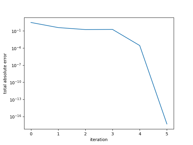
Example 1: Small diagonal matrix

In our first example, we construct a 5x5 diagonal matrix with 3 eigenvalues around 10, 1 eigenvalue equal to 2, and 1 equal to 1:

A = zeros(5,5)
A[1,1] = 10
A[2,2] = 10.1
A[3,3] = 10.2
A[4,4] = 2
A[5,5] = 1

Running the conjugate gradient, the algorithm terminates in 5 steps. We examine the error in the residual by computing the sum of the absolute residual components. Note that this is not the error in the solution but rather the error in the system. We see that the error drops sharply at 4 iterations, and then again in the 5th iteration.

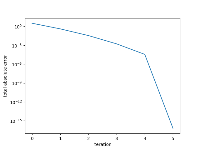
Example 2: Small random s.p.d. matrix

In our next example, we construct a 5x5 random s.p.d. matrix:

A = rand(5,5)
A = 0.5*(A+A')
A = A + 5*I

with, in this particular instance, eigenvalues

> eigvals(A)

5-element Array{Float64,1}:
 4.46066817714894
 4.979395596044116
 5.2165679905921785
 5.56276039133931
 7.909981699390226

Here the error drops sharply at the 5th iteration, reaching the desired convergence tolerance.

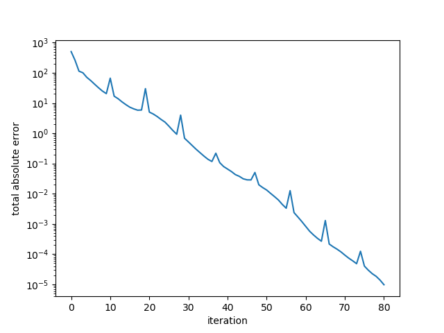
Example 3: Large random s.p.d. matrix (smaller condition number)

Next, we examine a matrix of dimension 1000, and generate a random s.p.d matrix.

A = rand(N,N)
A = 0.5*(A+A')
A = A + 50*I

Note that in the above snippet, the last line adds a large term to the diagonal, making the matrix “more nonsingular.” The condition number is:

> cond(A)

14.832223763483976

The general rule of thumb is that we lose about 1 digit of accuracy with condition numbers on this order.

The absolute error of the residual is plotted against iteration. Here the algorithm terminated in 11 iterations.

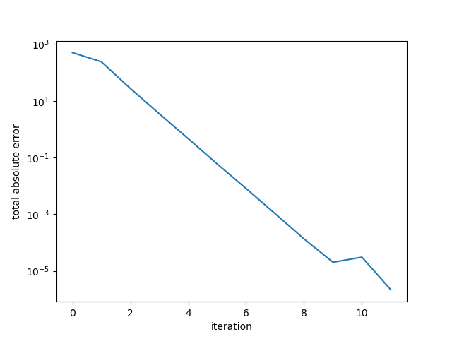
Example 4: Large random s.p.d. matrix (larger condition number)

Now we examine a matrix again of size 1000 but this time with a smaller multiplier on the diagonal (here we picked the smallest integer value such that the eigenvalues of the resulting matrix were all nonnegative):

A = rand(N,N)
A = 0.5*(A+A')
A = A + 13*I

The condition number is much larger than the previous case, almost at \(10^3\):

> cond(A)

2054.8953570922145

The error plot is below:

Here, the algorithm converged after 80 iterations. A quick check of the “conjugate” vectors shows that the set of vectors is indeed not conjugate.

Code on Github

A Jupyter notebook with all of the code (running Julia v1.0) is available on Github.

References

1. Shewchuk. An Introduction to Conjugate Gradient without the Agonizing Pain.
2. Nocedal and Wright. Numerical Optimization, Chapter 5.
3. Trefethen and Bau. Numerical Linear Algebra, Chapter 6.